legend
Add legend to axes
Syntax
Description
legend creates a legend with descriptive labels for each
plotted data series. For the labels, the legend uses the text from the
DisplayName properties of the data series. If the
DisplayName property is empty, then the legend uses a
label of the form 'dataN'. The legend automatically updates
when you add or delete data series from the axes. This command creates a legend
in the current axes, which is returned by the gca command. If
the current axes is empty, then the legend is empty. If no axes exist, then
legend creates a Cartesian axes.
legend( sets the
legend labels. Specify the labels as a list of character vectors or strings,
such as label1,...,labelN)legend('Jan','Feb','Mar').
legend( sets the labels using
a cell array of character vectors, a string array, or a character matrix, such
as labels)legend({'Jan','Feb','Mar'}).
legend( only
includes items in the legend for the data series listed in
subset,___)subset. Specify subset as a vector of
graphics objects. You can specify subset before specifying
the labels or with no other input arguments.
legend(___,'Location',
sets the legend location. For example, lcn)'Location','northeast'
positions the legend in the upper right corner of the axes. Specify the location
after other input arguments.
legend(___,'Orientation',,
where ornt)ornt is 'horizontal', displays the
legend items side-by-side. The default for ornt is
'vertical', which stacks the items vertically.
legend(___,
sets legend properties using one or more name-value pair arguments.Name,Value)
legend(, where
bkgd)bkgd is 'boxoff', removes the legend
background and outline. The default for bkgd is
'boxon', which displays the legend background and
outline.
lgd = legend(___)Legend object. Use
lgd to query and set properties of the legend after it is
created. For a list of properties, see Legend Properties.
legend( controls the visibility
of the legend, where vsbl)vsbl is 'hide',
'show', or 'toggle'.
legend('off') deletes the legend.
Examples
Add Legend to Current Axes
Plot two lines and add a legend to the current axes. Specify the legend labels as input arguments to the legend function.
x = linspace(0,pi);
y1 = cos(x);
plot(x,y1)

hold on
y2 = cos(2*x);
plot(x,y2)

legend('cos(x)','cos(2x)')

If you add or delete a data series from the axes, the legend updates accordingly. Control the label for the new data series by setting the DisplayName property as a name-value pair during creation. If you do not specify a label, then the legend uses a label of the form 'dataN'.
Note: If you do not want the legend to automatically update when data series are added to or removed from the axes, then set the AutoUpdate property of the legend to 'off'.
y3 = cos(3*x);
plot(x,y3,'DisplayName','cos(3x)')
hold off
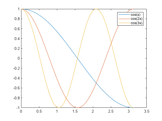
Delete the legend.
legend('off')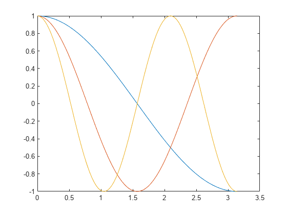
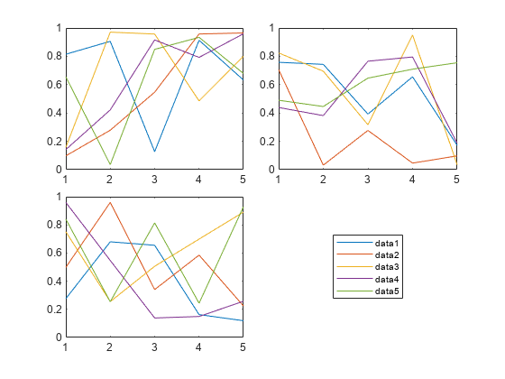
Add Legend to Specific Axes
Starting in R2019b, you can display a tiling of plots using the tiledlayout and nexttile functions. Call the tiledlayout function to create a 2-by-1 tiled chart layout. Call the nexttile function to create the axes objects ax1 and ax2. Plot random data in each axes. Add a legend to the upper plot by specifying ax1 as the first input argument to legend.
tiledlayout(2,1)
y1 = rand(3);
ax1 = nexttile;
plot(y1)

y2 = rand(5);
ax2 = nexttile;
plot(y2)

legend(ax1,{'Line 1','Line 2','Line 3'})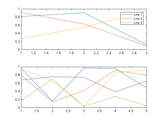
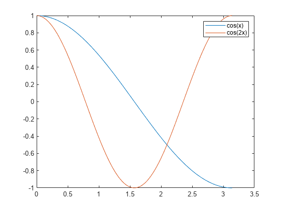
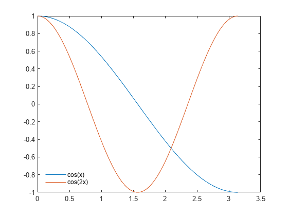
Specify Legend Labels During Plotting Commands
Plot two lines. Specify the legend labels during the plotting commands by setting the DisplayName property to the desired text. Then, add a legend.
x = linspace(0,pi);
y1 = cos(x);
plot(x,y1,'DisplayName','cos(x)')

hold on
y2 = cos(2*x);
plot(x,y2,'DisplayName','cos(2x)')
hold off

legend
Exclude Line from Legend
To exclude a line from the legend, specify its label as an empty character vector or string. For example, plot two sine waves, and add a dashed zero line by calling the yline function. Then create a legend, and exclude the zero line by specifying its label as ''.
x = 0:0.2:10;
plot(x,sin(x),x,sin(x+1));
hold on
yline(0,'--')
legend('sin(x)','sin(x+1)','')
List Entries in Columns and Specify Legend Location
Plot four lines. Create a legend in the northwest area of the axes. Specify the number of legend columns using the NumColumns property.
x = linspace(0,pi);
y1 = cos(x);
plot(x,y1)

hold on
y2 = cos(2*x);
plot(x,y2)

y3 = cos(3*x);
plot(x,y3)

y4 = cos(4*x);
plot(x,y4)
hold off

legend({'cos(x)','cos(2x)','cos(3x)','cos(4x)'},...
    'Location','northwest','NumColumns',2)
By default, the legend orders the items from top to bottom along each column. To order the items from left to right along each row instead, set the Orientation property to 'horizontal'.
Reverse Order of Legend Items
Since R2023b
You can reverse the order of the legend items by setting the Direction property of the legend. For example, plot four lines and add a legend.
plot([4 5 6 7; 0 1 2 3])
lgd = legend("First","Second","Third","Fourth");

Reverse the order of the legend items.
lgd.Direction = "reverse";
Display Shared Legend in Tiled Chart Layout
When you want to share a legend between two or more plots, you can display the legend in a separate tile of the layout. You can place the legend within the grid of tiles, or in an outer tile.
Create three plots in a tiled chart layout.
t = tiledlayout('flow','TileSpacing','compact');
nexttile
plot(rand(5))
nexttile
plot(rand(5))
nexttile
plot(rand(5))
Add a shared legend, and move it to the fourth tile.
lgd = legend;
lgd.Layout.Tile = 4;
Next, add a fourth plot and move the legend to the east tile.
nexttile
plot(rand(5))
lgd.Layout.Tile = 'east';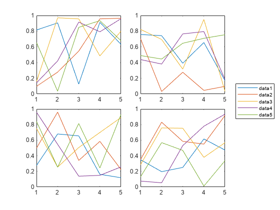
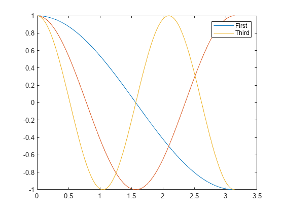
Included Subset of Graphics Objects in Legend
If you do not want to include all of the plotted graphics objects in the legend, then you can specify the graphics objects that you want to include.
Plot three lines and return the Line objects created. Create a legend that includes only two of the lines. Specify the first input argument as a vector of the Line objects to include.
x = linspace(0,pi);
y1 = cos(x);
p1 = plot(x,y1);

hold on
y2 = cos(2*x);
p2 = plot(x,y2);

y3 = cos(3*x);
p3 = plot(x,y3);
hold off

legend([p1 p3],{'First','Third'})
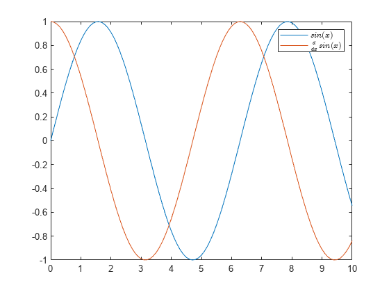
Create Legend with LaTeX Markup
Create a plot, and add a legend with LaTeX markup by calling the legend function and setting the Interpreter property to 'latex'. Surround the markup with dollar signs ($).
x = 0:0.1:10;
y = sin(x);
dy = cos(x);
plot(x,y,x,dy);
legend('$sin(x)$','$\frac{d}{dx}sin(x)$','Interpreter','latex');
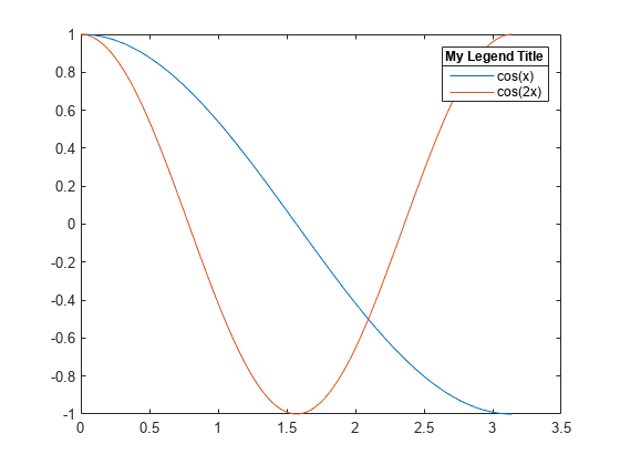
Add Title to Legend
Plot two lines and create a legend. Then, add a title to the legend.
x = linspace(0,pi);
y1 = cos(x);
plot(x,y1)

hold on
y2 = cos(2*x);
plot(x,y2)
hold off

lgd = legend('cos(x)','cos(2x)');
title(lgd,'My Legend Title')
Remove Legend Background
Plot two lines and create a legend in the lower left corner of the axes. Then, remove the legend background and outline.
x = linspace(0,pi);
y1 = cos(x);
plot(x,y1)

hold on
y2 = cos(2*x);
plot(x,y2)
hold off

legend({'cos(x)','cos(2x)'},'Location','southwest')
legend('boxoff')
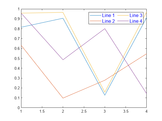
Specify Legend Font Size and Color
You can change different aspects of a legend by setting properties. You can set properties by specifying name-value arguments when you call legend, or you can set properties of the Legend object after you call legend.
Plot four lines of random data. Create a legend and assign the Legend object to the variable lgd. Set the FontSize and TextColor properties using name-value arguments.
rdm = rand(4);
plot(rdm)

lgd = legend({'Line 1','Line 2','Line 3','Line 4'},...
    'FontSize',12,'TextColor','blue');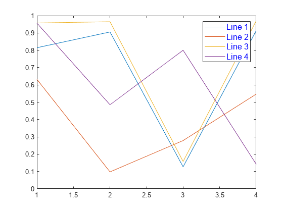
Modify the legend after it is created by referring to lgd. Set the NumColumns property using the object dot property name notation.
lgd.NumColumns = 2;
Input Arguments
label1,...,labelN — Labels (as separate arguments)
character vectors | strings
Labels, specified as a comma-separated list of character vectors or strings.
To exclude an item from the legend, specify the corresponding label as an empty character vector or string.
To include special characters or Greek letters in the labels, use TeX or
LaTeX markup. For a table of options, see the Interpreter property.
To specify labels that are keywords, such as 'Location'
or 'off', use a cell array of character vectors, a string
array, or a character array.
Example: legend('Sin Function','Cos
Function')
Example: legend("Sin Function","Cos
Function")
Example: legend("Sample A","","Sample C")
Example: legend('\gamma','\sigma')
labels — Labels (as an array)
cell array of character vectors | string array | categorical array
Labels, specified as a cell array of character vectors, string array, or categorical array.
To exclude an item from the legend, specify the corresponding label as an empty character vector in the cell array, or as an empty string in the string array.
To include special characters or Greek letters in the labels, use TeX or
LaTeX markup. For a table of options, see the Interpreter property.
Example: legend({'Sin Function','Cos
Function'})
Example: legend(["Sin Function","Cos
Function"])
Example: legend({'Sample A','','Sample
C'})
Example: legend({'\gamma','\sigma'})
Example: legend(categorical({'Alabama','New
York'}))
subset — Data series to include in legend
vector of graphics objects
Data series to include in the legend, specified as a vector of graphics objects.
target — Target for legend
Axes object |
PolarAxes object | GeographicAxes object | standalone visualization
Target for legend, specified as an Axes object, a
PolarAxes object, a GeographicAxes
object, or a standalone visualization with a
LegendVisible property, such as a
GeographicBubbleChart object. If you do not specify the
target, then the legend function uses the object returned
by the gca command as the target.
Standalone visualizations do not support modifying the legend appearance,
such as the location, or returning the Legend object as an
output argument..
lcn — Legend location
'north' | 'south' | 'east' | 'west' | 'northeast' | ...
Legend location with respect to the axes, specified as one of the location values listed in this table.
| Value | Description |
|---|---|
'north' | Inside top of axes |
'south' | Inside bottom of axes |
'east' | Inside right of axes |
'west' | Inside left of axes |
'northeast' | Inside top-right of axes (default for 2-D axes) |
'northwest' | Inside top-left of axes |
'southeast' | Inside bottom-right of axes |
'southwest' | Inside bottom-left of axes |
'northoutside' | Above the axes |
'southoutside' | Below the axes |
'eastoutside' | To the right of the axes |
'westoutside' | To the left of the axes |
'northeastoutside' | Outside top-right corner of the axes (default for 3-D axes) |
'northwestoutside' | Outside top-left corner of the axes |
'southeastoutside' | Outside bottom-right corner of the axes |
'southwestoutside' | Outside bottom-left corner of the axes |
'best' | Inside axes where least conflict occurs with the plot data at the time that you create the
legend. If the plot data changes, you might need to
reset the location to 'best'. |
'bestoutside' | Outside top-right corner of the axes (when the legend has a vertical orientation) or below the axes (when the legend has a horizontal orientation) |
'layout' | A tile in a tiled chart layout. To move the legend to
a different tile, set the Layout
property of the legend. |
'none' | Determined by Position property. Use the Position property
to display the legend in a custom location. |
Example: legend('Location','northeastoutside')
ornt — Orientation
'vertical' (default) | 'horizontal'
Orientation, specified as one of these values:
'vertical'— Stack the legend items vertically.'horizontal'— List the legend items side-by-side.
Example: legend('Orientation','horizontal')
bkgd — Legend box display
'boxon' (default) | 'boxoff'
Legend box display, specified as one of these values:
'boxon'— Display the legend background and outline.'boxoff'— Do not display the legend background and outline.
Example: legend('boxoff')
vsbl — Legend visibility
'hide' | 'show' | 'toggle'
Legend visibility, specified as one of these values:
'hide'— Hide the legend.'show'— Show the legend or create a legend if one does not exist.'toggle'— Toggle the legend visibility.
Example: legend('hide')
Name-Value Arguments
Specify optional pairs of arguments as
Name1=Value1,...,NameN=ValueN, where Name is
the argument name and Value is the corresponding value.
Name-value arguments must appear after other arguments, but the order of the
pairs does not matter.
Before R2021a, use commas to separate each name and value, and enclose
Name in quotes.
Example: legend({'A','B'},'TextColor','blue','FontSize',12)
creates a legend with blue, 12-point font.
Note
The properties listed here are only a subset. For a complete list, see Legend Properties.
Text color, specified as an RGB triplet, a hexadecimal color code, a color name, or a short
name. The default color is black with a value of [0 0 0].
For a custom color, specify an RGB triplet or a hexadecimal color code.
An RGB triplet is a three-element row vector whose elements specify the intensities of the red, green, and blue components of the color. The intensities must be in the range
[0,1], for example,[0.4 0.6 0.7].A hexadecimal color code is a string scalar or character vector that starts with a hash symbol (
#) followed by three or six hexadecimal digits, which can range from0toF. The values are not case sensitive. Therefore, the color codes"#FF8800","#ff8800","#F80", and"#f80"are equivalent.
Alternatively, you can specify some common colors by name. This table lists the named color options, the equivalent RGB triplets, and hexadecimal color codes.
| Color Name | Short Name | RGB Triplet | Hexadecimal Color Code | Appearance |
|---|---|---|---|---|
"red" | "r" | [1 0 0] | "#FF0000" |
|
"green" | "g" | [0 1 0] | "#00FF00" |
|
"blue" | "b" | [0 0 1] | "#0000FF" |
|
"cyan"
| "c" | [0 1 1] | "#00FFFF" |
|
"magenta" | "m" | [1 0 1] | "#FF00FF" |
|
"yellow" | "y" | [1 1 0] | "#FFFF00" |
|
"black" | "k" | [0 0 0] | "#000000" |
|
"white" | "w" | [1 1 1] | "#FFFFFF" |
|
"none" | Not applicable | Not applicable | Not applicable | No color |
Here are the RGB triplets and hexadecimal color codes for the default colors MATLAB® uses in many types of plots.
| RGB Triplet | Hexadecimal Color Code | Appearance |
|---|---|---|
[0 0.4470 0.7410] | "#0072BD" |
|
[0.8500 0.3250 0.0980] | "#D95319" |
|
[0.9290 0.6940 0.1250] | "#EDB120" |
|
[0.4940 0.1840 0.5560] | "#7E2F8E" |
|
[0.4660 0.6740 0.1880] | "#77AC30" |
|
[0.3010 0.7450 0.9330] | "#4DBEEE" |
|
[0.6350 0.0780 0.1840] | "#A2142F" |
|
Example: [0 0 1]
Example: 'blue'
Example: '#0000FF'
Output Arguments
Tips
To label more than 50 objects in the legend, specify a label for each object. Otherwise,
legenddepicts only the first 50 objects in the graph.
Algorithms
Recalling the
legendfunction does not reset legend properties, such as the location or orientation. If a legend exists, then thelegendfunction updates the existing legend. AnAxesobject can have only one legend.The legend reflects the visibility of graphics objects in the axes. Graphics objects that have a
Visibleproperty set to'off'appear as grayed out items in the legend.
Version History
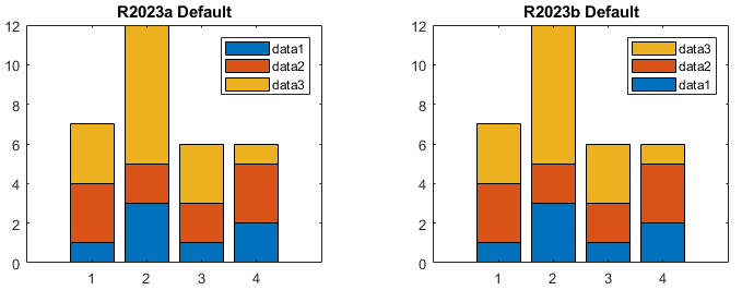
Introduced before R2006aR2023b: Legend order is reversed for stacked bar charts and area charts
The default order of legend items for stacked (vertical) bar charts and area charts is now reversed to match the stacking order of the chart. Previously, the legend items were listed in the opposite order of stacked bars and area charts.
To preserve the order of previous releases, set the Direction
property of the legend to "normal".
R2021a: Passing an empty label to the legend function omits the entry from the legend
When you call the legend function and specify a label as an
empty character vector, an empty string, or an empty element in a cell array or
string array, the corresponding entry is omitted from the legend. In R2020b and
earlier releases, the entry appears in the legend without a label.
For example, this code plots two sine waves and a reference line at
y=0. Then it creates a legend with three labels, where the
last label is empty. In R2020b, the third line appears in the legend without a
label. In R2021a, the third line is omitted from the legend.
x = 0:0.2:10;
plot(x,sin(x),x,sin(x+1));
hold on
yline(0,'--')
legend('sin(x)','sin(x+1)','')
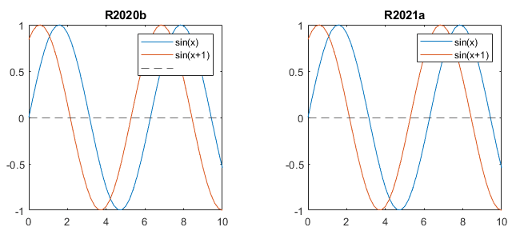
To keep an entry in the legend without a label, include a space character in the
label. For example, to update the preceding code, specify the last label as a
character vector containing a space ('
').
legend('sin(x)','sin(x+1)',' ')
Alternatively, if you do not want to display a space character, you can pass the
individual line objects to the legend function with an array of
labels. To get the individual line objects, call each plotting function with an
output
argument.
x = 0:0.2:10;
p = plot(x,sin(x),x,sin(x+1));
hold on
line0 = yline(0,'--');
legend([p(1) p(2) line0], {'sin(x)','sin(x+1)',''});
See Also
Functions
Properties
Topics
You can also select a web site from the following list:
Americas
- América Latina (Español)
- Canada (English)
- United States (English)
Europe
- Belgium (English)
- Denmark (English)
- Deutschland (Deutsch)
- España (Español)
- Finland (English)
- France (Français)
- Ireland (English)
- Italia (Italiano)
- Luxembourg (English)
- Netherlands (English)
- Norway (English)
- Österreich (Deutsch)
- Portugal (English)
- Sweden (English)
- Switzerland
- United Kingdom (English)