Differential Pulse Code Modulation

Scalar quantization uses methods that require no prior knowledge about the transmitted signal. In practice, you can often make educated guesses about the present signal based on past signal transmissions. Using educated guesses to help quantize a signal is known as predictive quantization. Differential pulse code modulation (DPCM) is the most common predictive quantization method. The dpcmenco, dpcmdeco, and dpcmopt functions can help you implement a DPCM predictive quantizer with a linear predictor.

Represent Predictors

To determine a DPCM encoder for a quantizer, you must supply not only a partition and codebook as described in Quantization, but also a predictor. The predictor is a function that the DPCM encoder uses to produce the educated guess at each step. A linear predictor has the form

y(k) = p(1)x(k-1) + p(2)x(k-2) + ... + p(m-1)x(k-m+1) + p(m)x(k-m)

where x is the original signal, y(k) attempts to predict the value of x(k), and p is an m-tuple of real numbers. Instead of quantizing x itself, the DPCM encoder quantizes the predictive error, x-y. The integer m above is called the predictive order. The special case when m = 1 is called delta modulation.

Suppose the guess for the kth value of the signal x, based on earlier values of x, as follows:

y(k) = p(1)x(k-1) + p(2)x(k-2) +...+ p(m-1)x(k-m+1) + p(m)x(k-m)

Then the corresponding predictor vector for toolbox functions is this vector:

predictor = [0, p(1), p(2), p(3),..., p(m-1), p(m)]

Note

The initial zero in the predictor vector makes sense if you view the vector as the polynomial transfer function of a finite impulse response (FIR) filter.

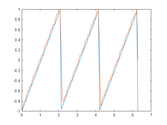
DPCM Encoding and Decoding

This example implements a simple case of DPCM that quantizes the difference between the value of the current signal sample and the value of the previous sample. For this case, the predictor is just y(k) = x (k - 1). It then encodes a sawtooth signal, decodes it, plots both the original and the decoded signals, and computes the mean square error between the original and decoded signals.

partition = [-1:.1:.9];
codebook = [-1:.1:1];
predictor = [0 1];      % y(k)=x(k-1)
t = [0:pi/50:2*pi];     % Time samples
x = sawtooth(3*t);      % Original signal

Quantize x using DPCM encoding.

encodedx = dpcmenco(x,codebook,partition,predictor);

Try to recover x from the modulated signal by using DPCM decoding. Plot the original signal and the decoded signal. The solid line is the original signal, while the dashed line is the recovered signal.

decodedx = dpcmdeco(encodedx,codebook,predictor);
plot(t,x,t,decodedx,'-')

Compute the mean square error between the original signal and the decoded signal.

distor = sum((x-decodedx).^2)/length(x)

distor = 
0.0327

Optimize DPCM Parameters

To optimize a DPCM-encoded and -decoded sawtooth signal, use the dpcmopt function with the dpcmenco and dpcmdeco functions. Testing and selecting parameters for large signal sets with a fine quantization scheme can be tedious. One way to produce partition, codebook, and predictor parameters easily is to optimize them according to a set of training data. The training data should be typical of the kinds of signals to be quantized with dpcmenco.

This example uses the predictive order, 1, as the desired order of the new optimized predictor. The dpcmopt function creates these optimized parameters, using the sawtooth signal x as training data. The example goes on to quantize the training data itself. In theory, the optimized parameters are suitable for quantizing other data that is similar to x. The mean square distortion for optimized DPCM is much less than the distortion with nonoptimized DPCM parameters.

Define variables for a sawtooth signal and initial DPCM parameters.

t = [0:pi/50:2*pi];
x = sawtooth(3*t);
partition = [-1:.1:.9];
codebook = [-1:.1:1];
predictor = [0 1];      % y(k)=x(k-1)

Optimize the partition, codebook, and predictor vectors by using the dpcmopt function and the initial codebook and order 1. Then generate DPCM encoded signals by using the initial and the optimized partition and codebook vectors.

[predictorOpt,codebookOpt,partitionOpt] = dpcmopt(x,1,codebook);
encodedx = dpcmenco(x,codebook,partition,predictor);
encodedxOpt = dpcmenco(x,codebookOpt,partitionOpt,predictorOpt);

Try to recover x from the modulated signal by using DPCM decoding. Compute the mean square error between the original signal and the decoded and optimized decoded signals.

decodedx = dpcmdeco(encodedx,codebook,predictor);
decodedxOpt = dpcmdeco(encodedxOpt,codebookOpt,predictorOpt);
distor = sum((x-decodedx).^2)/length(x);
distorOpt = sum((x-decodedxOpt).^2)/length(x);

Compare mean square distortions for quantization with the initial and optimized input arguments.

[distor, distorOpt]

ans = 1×2

    0.0327    0.0009