Absolute Stability for Quantized System
This example shows how to enforce absolute stability when a linear time-invariant system is in feedback interconnection with a static nonlinearity that belongs to a conic sector.
Feedback Connection
Consider the feedback connection as shown in Figure 1.
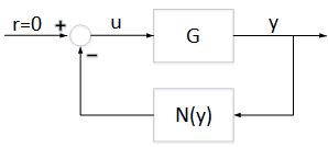
Figure 1: Feedback connection
 is a linear time invariant system, and
  is a static nonlinearity that belongs to a conic sector
 ![$[\alpha,\beta]$](../../examples/control/win64/AbsoluteStabilityForQuantizedSystemExample_eq17999177181437605090.png) (where
(where  ); that is,

For this example, is the following discrete-time system.
A = [0.9995, 0.0100, 0.0001;
    -0.0020, 0.9995, 0.0106;
          0,      0, 0.9978];
B = [0, 0.002, 0.04]';
C = [2.3948, 0.3303, 2.2726];
D = 0;
G = ss(A,B,C,D,0.01);
Sector Bounded Nonlinearity
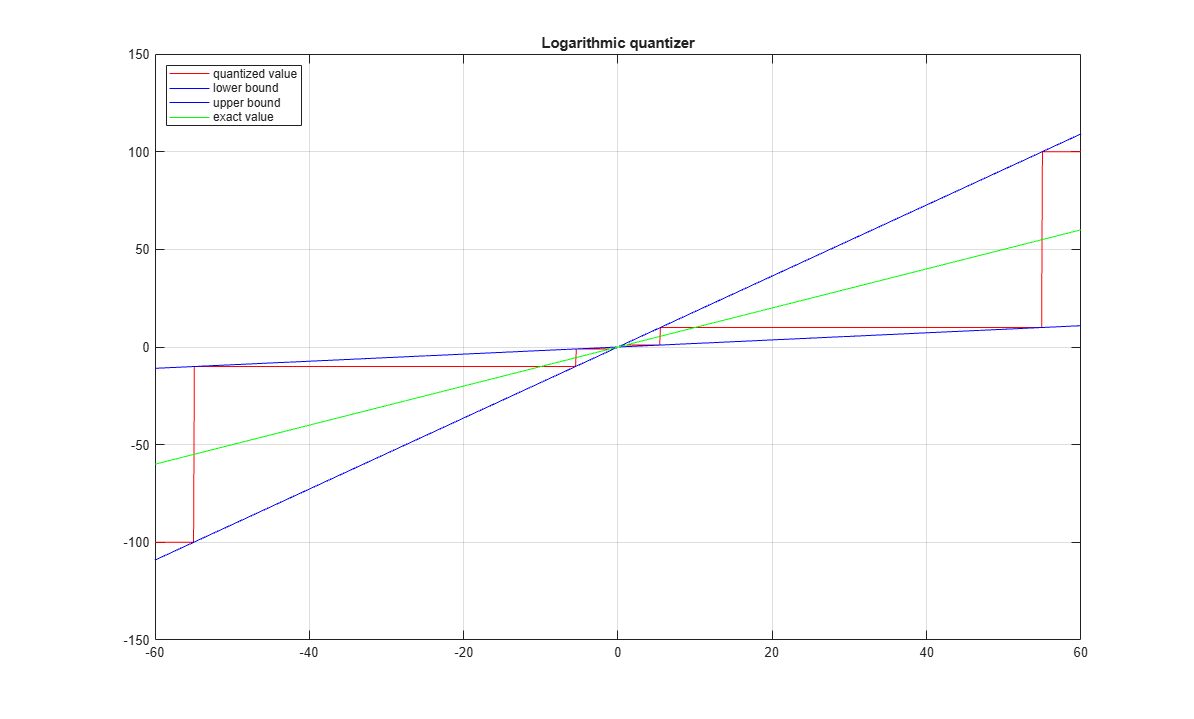
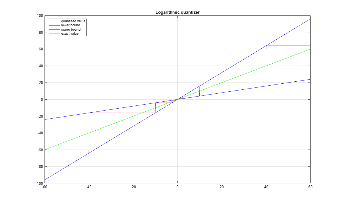
In this example, the nonlinearity is the logarithmic quantizer, which is defined as follows:

where,  . This quantizer belongs to a sector bound
 ![$[\frac{2\rho}{1+\rho},\frac{2}{1+\rho}]$](../../examples/control/win64/AbsoluteStabilityForQuantizedSystemExample_eq05936810714490360334.png) . For example, if
. For example, if  , then the quantizer belongs to the conic sector [0.1818,1.8182].
% Quantizer parameter
rho = 0.1;
% Lower bound
alpha = 2*rho/(1+rho)
% Upper bound
beta = 2/(1+rho)
alpha =

    0.1818


beta =

    1.8182
Plot the sector bounds for the quantizer.
PlotSectorBound(rho)
 represents the quantization density, where
  . If is larger, then the quantized value is more accurate. For more details about this quantizer, see [1].
Conic Sector Condition for Absolute Stability
The conic sector matrix for the quantizer is given by

To guarantee stability of the feedback connection in Figure 1, the linear system needs to satisfy

where,  and
and  are the input and output of , respectively.
This condition can be verified by checking if the sector index,  , is less than
 1.
Define the conic sector matrix for a quantizer with .
Q = [1,-(alpha+beta)/2;-(alpha+beta)/2,alpha*beta];
Get the sector index for Q and G.
R = getSectorIndex([1;-G],-Q)
R =

    1.8247
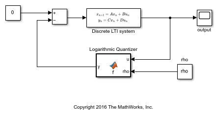
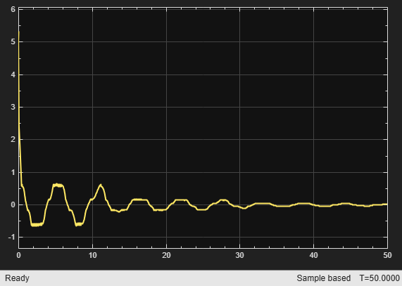
Since  , the closed-loop system is not stable. To see this instability, use the following Simulink® model.
mdl = 'DTQuantization';
open_system(mdl)
Run the Simulink model.
sim(mdl)
open_system('DTQuantization/output')
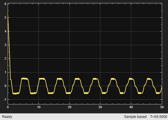
From the output trajectory, it can be seen that the closed-loop system is not stable. This is because the quantizer with is too coarse.
Increase the quantization density by letting  . The quantizer belongs to the conic sector [0.4,1.6].
% Quantizer parameter
rho = 0.25;
% Lower bound
alpha = 2*rho/(1+rho)
% Upper bound
beta = 2/(1+rho)
alpha =

    0.4000


beta =

    1.6000
Plot the sector bounds for the quantizer.
PlotSectorBound(rho)
Define the conic sector matrix for a quantizer with .
Q = [1,-(alpha+beta)/2;-(alpha+beta)/2,alpha*beta];
Get the sector index for Q and G.
R = getSectorIndex([1;-G],-Q)
R =

    0.9702
The quantizer with satisfies the conic sector condition for stability of the feedback connection since  .
.
Run the Simulink model with .
sim(mdl)
open_system('DTQuantization/output')
As indicated by the sector index, the closed-loop system is stable.
Reference
[1] M. Fu and L. Xie,"The sector bound approach to quantized feedback control," IEEE Transactions on Automatic Control 50(11), 2005, 1698-1711.