regARIMA Model Estimation Using Equality Constraints

estimate requires a regARIMA model and a vector of univariate response data to estimate a regression model with ARIMA errors. Without predictor data, the model specifies the parametric form of an intercept-only regression component with an ARIMA error model. This is not the same as a conditional mean model with a constant. For details, see Alternative ARIMA Model Representations. If you specify a $\mathit{T}$-by-$\mathit{r}$ matrix of predictor data, then estimate includes a linear regression component for the $\mathit{r}$ series.

estimate returns fitted values for any parameters in the input model with NaN values. For example, if you specify a default regARIMA model and pass a $\mathit{T}$-by-$\mathit{r}$ matrix of predictor data, then the software sets all parameters to NaN including the $\mathit{r}$ regression coefficients, and estimates them all. If you specify non-NaN values for any parameters, then estimate views these values as equality constraints and honors them during estimation.

For example, suppose residual diagnostics from a linear regression suggest integrated unconditional disturbances. Since the regression intercept is unidentifiable in integrated models, you decide to set the intercept to 0. Specify 'Intercept',0 in the regARIMA model that you pass into estimate. The software views this non-NaN value as an equality constraint, and does not estimate the intercept, its standard error, and its covariance with other estimates. To illustrate further, suppose the true model for a response series ${\mathit{y}}_{\mathit{t}}$ is

$$\begin{array}{l}{y}_t=0+u_t\\ u_t={\epsilon }_t,\end{array}$$

where ${\epsilon }_{\mathit{t}}$ is Gaussian with variance 1. The loglikelihood function for a simulated data set from this model can resemble the surface in the following figure over a grid of variances and intercepts.

rng(1); % For reproducibility
e = randn(100,1);
Variance = 1;
Intercept = 0;
Mdl0 = regARIMA('Intercept',Intercept,'Variance',Variance);
y = filter(Mdl0,e);

gridLength = 25;
intGrid1 = linspace(-1,1,gridLength);
varGrid1 = linspace(0.1,4,gridLength);
[varGrid2,intGrid2] = meshgrid(varGrid1,intGrid1);
LogLGrid = zeros(numel(varGrid1),numel(intGrid1));

for k1 = 1:numel(intGrid1)
    for k2 = 1:numel(varGrid1)
        Mdl = regARIMA('Intercept',...
            intGrid1(k1),'Variance',varGrid1(k2));
        [~,~,LogLGrid(k1,k2)] = estimate(Mdl,y,'Display','off');
    end
end

figure
surf(intGrid2,varGrid2,LogLGrid) % 3D loglikelihood plot        
xlabel 'Intercept';
ylabel 'Variance';
zlabel 'Loglikelihood';
shading interp

Notice that the maximum (yellow region) occurs around where the intercept is 0 and the variance is 1. If you apply an equality constraint, then the optimizer views a two-dimensional slice (in this example) of the loglikelihood function at that constraint. The following plots display the loglikelihood at several different equality constraints on the intercept.

intValue = [intGrid1(5), intGrid1(10),...
    intGrid1(15), intGrid1(20)];

figure
for k = 1:4
    subplot(2,2,k)
    plot(varGrid1,LogLGrid(intGrid2 == intValue(k)))
    title(sprintf('Loglikelihood, Intercpet = %.3f',intValue(k)))
    xlabel 'Variance';
    ylabel 'Loglikelihood';
    hold on
    h1 = gca;
    plot([Variance Variance],h1.YLim,'r:')
    hold off
end

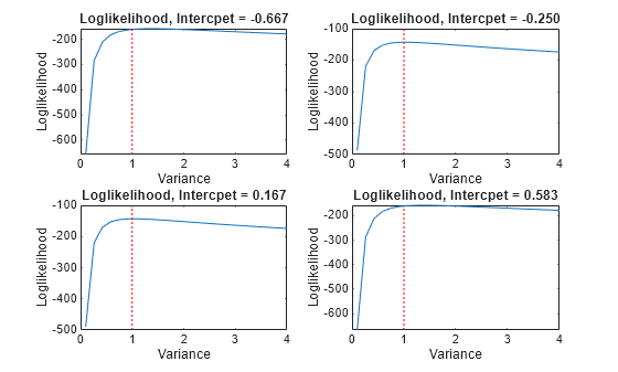
In each case, the maximum of the loglikelihood function occurs close to the true value of the variance.

Rather than constrain the intercept, the following plots display the likelihood function using several equality constraints on the variance.

varValue = [varGrid1(5),varGrid1(10),varGrid1(15),varGrid1(20)];

figure
for k = 1:4
    subplot(2,2,k)
    plot(intGrid1,LogLGrid(varGrid2 == varValue(k)))
    title(sprintf('Loglikelihood, Variance = %.3f',varValue(k)))
    xlabel('Intercept')
    ylabel('Loglikelihood')
    hold on
    h2 = gca;
    plot([Intercept Intercept],h2.YLim,'r:')
    hold off
end

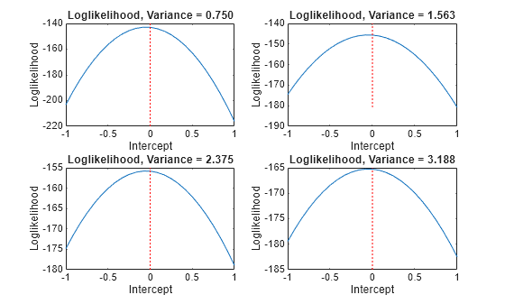
In each case, the maximum of the loglikelihood function occurs close to the true value of the intercept.

estimate also honors a subset of equality constraints while estimating all other parameters set to NaN. For example, suppose $\mathit{r}=3$, and you know that ${\beta }_2=5$. Specify Beta = [NaN; 5; NaN] in the regARIMA model, and pass this model with the data to estimate.

estimate optionally returns the estimated covariance matrix for the estimated parameters. If any parameter known to the optimizer has an equality constraint, then the corresponding row and column of the variance-covariance matrix is composed of zeros.