Specify Gradient for HMC Sampler
This example shows how to set up a Bayesian linear regression model for efficient posterior sampling using the Hamiltonian Monte Carlo (HMC) sampler. The prior distribution of the coefficients is a multivariate t, and the disturbance variance has an inverse gamma prior.
Consider the multiple linear regression model that predicts U.S. real gross national product (GNPR) using a linear combination of industrial production index (IPI), total employment (E), and real wages (WR).

For all  ,
,  is a series of independent Gaussian disturbances with a mean of 0 and variance
  . Assume these prior distributions.
 is a 4-D t distribution with 30 degrees of freedom for each component, correlation matrix
 C, locationct, and scalest.
 , with shape
  and scale
  .
.
bayeslm treats these assumptions and the data likelihood as if the corresponding posterior is analytically intractable.
Declare a MATLAB® function that:
Accepts values of
 and together in a column vector, and accepts values of the hyperparameters.
Returns the log of the joint prior distribution,
 , given the values of and , and returns the gradient of the log prior density with respect to and
  .
.
function [logPDF,gradient] = priorMVTIGHMC(params,ct,st,dof,C,a,b)
%priorMVTIGHMC Log density of multivariate t times inverse gamma and
%gradient
%   priorMVTIGHMC passes params(1:end-1) to the multivariate t density
%   function with dof degrees of freedom for each component and positive
%   definite correlation matrix C, and passes params(end) to the inverse
%   gamma distribution with shape a and scale b.  priorMVTIG returns the
%   log of the product of the two evaluated densities and its gradient.
%   After applying the log, terms involving constants only are dropped from
%   logPDF.
%
%   params: Parameter values at which the densities are evaluated, an
%           m-by-1 numeric vector.
%
%       ct: Multivariate t distribution component centers, an (m-1)-by-1
%           numeric vector.  Elements correspond to the first m-1 elements
%           of params.
%
%       st: Multivariate t distribution component scales, an (m-1)-by-1
%           numeric vector.  Elements correspond to the first m-1 elements
%           of params.
%
%      dof: Degrees of freedom for the multivariate t distribution, a
%           numeric scalar or (m-1)-by-1 numeric vector. priorMVTIG expands
%           scalars such that dof = dof*ones(m-1,1). Elements of dof
%           correspond to the elements of params(1:end-1).
%
%        C: correlation matrix for the multivariate t distribution, an
%           (m-1)-by-(m-1) symmetric, positive definite matrix. Rows and
%           columns correspond to the elements of params(1:end-1).
%
%        a: Inverse gamma shape parameter, a positive numeric scalar.
%
%        b: Inverse gamma scale parameter, a positive scalar.
%
beta = params(1:(end-1));
numCoeffs = numel(beta);
sigma2 = params(end);

tVal = (beta - ct)./st;
expo = -(dof + numCoeffs)/2;
logmvtDensity = expo*log(1 + (1/dof)*((tVal'/C)*tVal));
logigDensity = (-a - 1)*log(sigma2) - 1/(sigma2*b);
logPDF = logmvtDensity + logigDensity;

grad_beta = (expo/(1 + (1/dof)*(tVal'/C*tVal)))*((2/dof)*((tVal'/C)'./st));
grad_sigma = (-a - 1)/sigma2 + 1/(sigma2^2*b);
gradient = [grad_beta; grad_sigma];
end
Create an anonymous function that operates like priorMVTIGHMC, but accepts the parameter values only and holds the hyperparameter values fixed at arbitrarily chosen values.
rng(1); % For reproducibility
dof = 30;
V = rand(4,4);
Sigma = V'*V;
st = sqrt(diag(Sigma));
C = Sigma./(st*st');
ct = -10*rand(4,1);
a = 10*rand;
b = 10*rand;
logPDF = @(params)priorMVTIGHMC(params,ct,st,dof,C,a,b);
Create a custom joint prior model for the linear regression parameters. Specify the number of predictors, p. Also, specify the function handle for priorMVTIGHMC and the variable names.
p = 3;
PriorMdl = bayeslm(p,'ModelType','custom','LogPDF',logPDF,...
    'VarNames',["IPI" "E" "WR"]);
PriorMdl is a customblm Bayesian linear regression model object representing the prior distribution of the regression coefficients and disturbance variance.
Load the Nelson-Plosser data set. Create variables for the response and predictor series. For numerical stability, convert the series to returns.
load Data_NelsonPlosser
X = price2ret(DataTable{:,PriorMdl.VarNames(2:end)});
y = price2ret(DataTable{:,'GNPR'});
Estimate the marginal posterior distributions of and using the HMC sampler. To monitor the progress of the sampler, specify a verbosity level of 2. For numerical stability, specify reparameterization of the disturbance variance.
options = sampleroptions('Sampler','hmc','VerbosityLevel',2)
PosteriorMdl = estimate(PriorMdl,X,y,'Options',options,'Reparameterize',true);
options =

  struct with fields:

                        Sampler: 'HMC'
           StepSizeTuningMethod: 'dual-averaging'
         MassVectorTuningMethod: 'iterative-sampling'
    NumStepSizeTuningIterations: 100
          TargetAcceptanceRatio: 0.6500
                  NumStepsLimit: 2000
                 VerbosityLevel: 2
                       NumPrint: 100

o Tuning mass vector using method: iterative-sampling

o Initial step size for dual-averaging = 0.0625

|==================================================================================|
|   ITER   |    LOG PDF    |  STEP SIZE  |  NUM STEPS  |  ACC RATIO  |  DIVERGENT  |
|==================================================================================|
|      100 |  4.084850e+01 |   9.102e-02 |          55 |   6.300e-01 |           2 |
Finished mass vector tuning iteration 1 of 5.

o Initial step size for dual-averaging = 0.5

|==================================================================================|
|   ITER   |    LOG PDF    |  STEP SIZE  |  NUM STEPS  |  ACC RATIO  |  DIVERGENT  |
|==================================================================================|
|      100 |  4.222442e+01 |   5.154e-01 |          10 |   6.500e-01 |           0 |

|==================================================================================|
|   ITER   |    LOG PDF    |  STEP SIZE  |  NUM STEPS  |  ACC RATIO  |  DIVERGENT  |
|==================================================================================|
|      100 |  4.078962e+01 |   3.725e-02 |           6 |   8.000e-01 |           0 |
Finished mass vector tuning iteration 2 of 5.

o Initial step size for dual-averaging = 0.5

|==================================================================================|
|   ITER   |    LOG PDF    |  STEP SIZE  |  NUM STEPS  |  ACC RATIO  |  DIVERGENT  |
|==================================================================================|
|      100 |  3.676157e+01 |   2.791e-01 |          18 |   6.300e-01 |           0 |

|==================================================================================|
|   ITER   |    LOG PDF    |  STEP SIZE  |  NUM STEPS  |  ACC RATIO  |  DIVERGENT  |
|==================================================================================|
|      100 |  3.826446e+01 |   2.512e-01 |           4 |   7.950e-01 |           0 |
|      200 |  4.089424e+01 |   1.031e-01 |          16 |   8.567e-01 |           0 |
Finished mass vector tuning iteration 3 of 5.

o Initial step size for dual-averaging = 0.25

|==================================================================================|
|   ITER   |    LOG PDF    |  STEP SIZE  |  NUM STEPS  |  ACC RATIO  |  DIVERGENT  |
|==================================================================================|
|      100 |  4.256806e+01 |   3.299e-01 |          15 |   6.500e-01 |           0 |

|==================================================================================|
|   ITER   |    LOG PDF    |  STEP SIZE  |  NUM STEPS  |  ACC RATIO  |  DIVERGENT  |
|==================================================================================|
|      100 |  4.268094e+01 |   1.663e-02 |           2 |   7.900e-01 |           0 |
|      200 |  3.925843e+01 |   2.969e-01 |          15 |   8.500e-01 |           0 |
Finished mass vector tuning iteration 4 of 5.

o Initial step size for dual-averaging = 0.25

|==================================================================================|
|   ITER   |    LOG PDF    |  STEP SIZE  |  NUM STEPS  |  ACC RATIO  |  DIVERGENT  |
|==================================================================================|
|      100 |  4.294744e+01 |   3.210e-01 |          16 |   6.200e-01 |           0 |

|==================================================================================|
|   ITER   |    LOG PDF    |  STEP SIZE  |  NUM STEPS  |  ACC RATIO  |  DIVERGENT  |
|==================================================================================|
|      100 |  4.041877e+01 |   9.263e-02 |           4 |   7.750e-01 |           0 |
|      200 |  4.199693e+01 |   2.889e-01 |           5 |   8.400e-01 |           0 |
Finished mass vector tuning iteration 5 of 5.

o Tuning step size using method: dual-averaging. Target acceptance ratio = 0.65

o Initial step size for dual-averaging = 0.5

|==================================================================================|
|   ITER   |    LOG PDF    |  STEP SIZE  |  NUM STEPS  |  ACC RATIO  |  DIVERGENT  |
|==================================================================================|
|      100 |  4.219634e+01 |   3.394e-01 |          15 |   6.400e-01 |           0 |

Method: MCMC sampling with 10000 draws
Number of observations: 61
Number of predictors:   4

           |   Mean     Std         CI95        Positive  Distribution
-----------------------------------------------------------------------
 Intercept |  0.0076  0.0087  [-0.009,  0.024]    0.806     Empirical
 IPI       | -0.1638  0.1453  [-0.469,  0.101]    0.122     Empirical
 E         |  2.3732  0.5434  [ 1.401,  3.532]    1.000     Empirical
 WR        | -0.2315  0.3020  [-0.838,  0.348]    0.218     Empirical
 Sigma2    |  0.0036  0.0007  [ 0.002,  0.005]    1.000     Empirical
PosteriorMdl is an empiricalblm model object storing the draws from the posterior distributions.
View trace plots and autocorrelation function (ACF) plots of the draws from the posteriors.
for j = 1:4
    figure;
    subplot(2,1,1)
    plot(PosteriorMdl.BetaDraws(j,:));
    title(sprintf('Trace plot - Beta %d',j));
    xlabel('MCMC draw')
    ylabel('Simulation index')
    subplot(2,1,2)
    autocorr(PosteriorMdl.BetaDraws(j,:))
end

figure;
subplot(2,1,1)
plot(PosteriorMdl.Sigma2Draws);
title('Trace plot - Disturbance Variance');
xlabel('MCMC draw')
ylabel('Simulation index')
subplot(2,1,2)
autocorr(PosteriorMdl.Sigma2Draws)
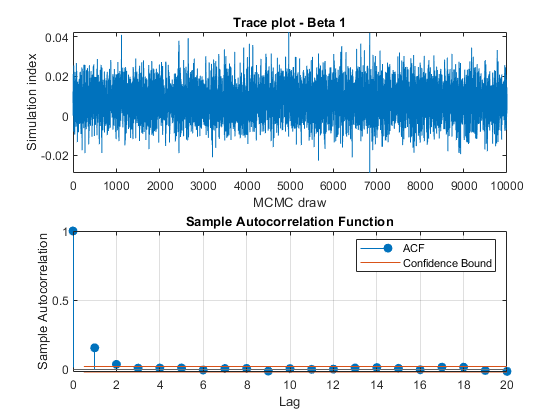
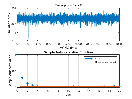

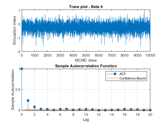
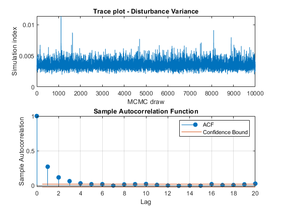
The trace plots show adequate mixing and no transient behavior. The autocorrelation plots show low correlation among subsequent samples.