Term Structure Calculations
Introduction
So far, a more formal definition of "yield" and its application has not been developed. In many situations when cash flow is available, discounting factors to the cash flows may not be immediately apparent. In other cases, what is relevant is often a spread, the difference between curves (also known as the term structure of spread).
All these calculations require one main ingredient, the Treasury spot, par-yield, or forward curve. Typically, the generation of these curves starts with a series of on-the-run and selected off-the-run issues as inputs.
MATLAB® software uses these bonds to find spot rates one at a time, from the shortest maturity onwards, using bootstrap techniques. All cash flows are used to construct the spot curve, and rates between maturities (for these coupons) are interpolated linearly.
Computing Spot and Forward Curves
This example shows how to compute spot and forward rates using zbtyield and zbtprice.
For an illustration of how this works, observe the use of zbtyield (or equivalently zbtprice) on a portfolio of six Treasury bills and bonds.
Bills | Maturity Date | Current Yield |
|---|---|---|
3 month | 4/17/03 | 1.15 |
6 month | 7/17/03 | 1.18 |
Notes/Bonds | Coupon | Maturity Date | Current Yield |
|---|---|---|---|
2 year | 1.750 | 12/31/04 | 1.68 |
5 year | 3.000 | 11/15/07 | 2.97 |
10 year | 4.000 | 11/15/12 | 4.01 |
30 year | 5.375 | 2/15/31 | 4.92 |
You can specify prices or yields to the bonds above to infer the spot curve. The function zbtyield accepts yields (bond-equivalent yield, to be exact).
To proceed, first assemble the above table into a variable called Bonds. The first column contains maturities, the second contains coupons, and the third contains notionals or face values of the bonds. (Note that bills have zero coupons.)
Bonds = [datenum('04/17/2003')    0        100;
         datenum('07/17/2003')    0        100;
         datenum('12/31/2004')    0.0175   100;
         datenum('11/15/2007')    0.03     100;
         datenum('11/15/2012')    0.04     100;
         datenum('02/15/2031')    0.05375  100];
Specify the corresponding yields.
Yields  = [0.0115;
           0.0118;
           0.0168;
           0.0297;
           0.0401;
           0.0492];
Compute the spot curve for each of these six maturities. The spot curve is based on a settlement date of January 17, 2003.
Settle = datenum('17-Jan-2003');
[ZeroRates, CurveDates] = zbtyield(Bonds, Yields, Settle)
ZeroRates = 6×1
0.0115
0.0118
0.0168
0.0302
0.0418
0.0550
CurveDates = 6×1

      731688
      731779
      732312
      733361
      735188
      741854
This is the Treasury spot curve for the day.
You can compute the forward curve from this spot curve with zero2fwd.
[ForwardRates, CurveDates] = zero2fwd(ZeroRates, CurveDates, ...
Settle)
ForwardRates = 6×1

    0.0115
    0.0121
    0.0185
    0.0394
    0.0530
    0.0621
CurveDates = 6×1

      731688
      731779
      732312
      733361
      735188
      741854
Here the notion of forward rates refers to rates between the maturity dates shown above, not to a certain period (forward 3-month rates, for example).

Copyright 2024 The MathWorks, Inc.
Computing Spreads
Calculating the spread between specific, fixed forward periods (such as the Treasury-Eurodollar spread) requires an extra step. Interpolate the zero rates (or zero prices, instead) for the corresponding maturities on the interval dates. Then use the interpolated zero rates to deduce the forward rates, and thus the spread of Eurodollar forward curve segments versus the relevant forward segments from Treasury bills.
Additionally, the variety of curve functions (including zero2fwd) helps to standardize such calculations.
For instance, by making both rates quoted with quarterly compounding
and on an actual/360 basis, the resulting spread structure is fully
comparable. This avoids the small inconsistency that occurs when directly
comparing the bond-equivalent yield of a Treasury bill to the quarterly
forward rates implied by Eurodollar futures.
Noise in Curve Computations
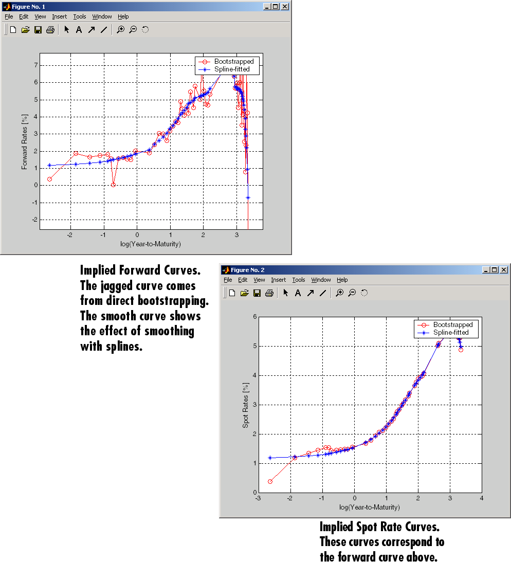
When introducing more bonds in constructing curves, noise may become a factor and may need some “smoothing” (with splines, for example); this helps obtain a smoother forward curve.
The following spot and forward curves are constructed from 67 Treasury bonds. The fitted and bootstrapped spot curve (bottom right figure) displays comparable stability. The forward curve (upper-left figure) contains significant noise and shows an improbable forward rate structure. The noise is not necessarily bad; it could uncover trading opportunities for a relative-value approach. Yet, a more balanced approach is desired when the bootstrapped forward curve oscillates this much and contains a negative rate as large as -10% (not shown in the plot because it is outside the limits).

This example uses termfit, an example function
from Financial Toolbox™ software that also requires the use of Curve Fitting Toolbox™ software.