Compute Square Root Using CORDIC
This example shows how to compute square root using a CORDIC kernel algorithm in MATLAB®. CORDIC-based algorithms are critical to many embedded applications, including motor controls, navigation, signal processing, and wireless communications.
CORDIC is an acronym for COordinate Rotation DIgital Computer. The Givens rotation-based CORDIC algorithm is one of the most hardware efficient algorithms because it only requires iterative shift-add operations [1,2]. The CORDIC algorithm eliminates the need for explicit multipliers and is suitable for calculating a variety of functions, such as sine, cosine, arcsine, arccosine, arctangent, vector magnitude, divide, square root, hyperbolic, and logarithmic functions.
The fixed-point CORDIC algorithm requires the following operations:
1 table lookup per iteration
2 shifts per iteration
3 additions per iteration
Note that for hyperbolic CORDIC-based algorithms, such as square root, certain iterations () are repeated to achieve result convergence [2].
CORDIC Kernel Algorithms Using Hyperbolic Computation Modes
You can use a CORDIC computing mode algorithm to calculate hyperbolic functions, such as hyperbolic trigonometric, square root, log, exp, etc.
CORDIC Equations in Hyperbolic Vectoring Mode
The hyperbolic vectoring mode is used for computing square root.
For the vectoring mode, the CORDIC equations are as follows:
where
is the sequence with repeated steps every iteration, and
if , and otherwise.
This mode provides the following result as approaches :
where
.
Note that the sequence in the product is repeated on each of the steps [2].
Typically is chosen to be a large-enough constant value. Thus, may be pre-computed.
Note also that for square root, only the result is used.
Implement a CORDIC Hyperbolic Vectoring Algorithm in MATLAB
A MATLAB code implementation example of the CORDIC hyperbolic vectoring kernel algorithm follows (for the case of scalar x, y, and z). This same code can be used for both fixed-point and floating-point data types.
CORDIC Hyperbolic Vectoring Kernel
k = 4; % Used for the repeated (3*k + 1) iteration steps
for idx = 1:N
    xtmp = bitsra(x, idx); % multiply by 2^(-idx)
    ytmp = bitsra(y, idx); % multiply by 2^(-idx)
    if y < 0
        x(:) = x + ytmp;
        y(:) = y + xtmp;
        z(:) = z - atanhLookupTable(idx);
    else
        x(:) = x - ytmp;
        y(:) = y - xtmp;
        z(:) = z + atanhLookupTable(idx);
    end
    if idx==k
        xtmp = bitsra(x, idx); % multiply by 2^(-idx)
        ytmp = bitsra(y, idx); % multiply by 2^(-idx)
        if y < 0
            x(:) = x + ytmp;
            y(:) = y + xtmp;
            z(:) = z - atanhLookupTable(idx);
        else
            x(:) = x - ytmp;
            y(:) = y - xtmp;
            z(:) = z + atanhLookupTable(idx);
        end
        k = 3*k + 1;
    end
end % idx loop
The hyperbolic inverse tangent lookup table atanhLookupTable is defined as follows, which in code generation is pre-computed and will be a constant.
atanhLookupTable = cast(atanh(2.^-(1:N)),'like',z);
Compute Square Root Using the CORDIC Hyperbolic Vectoring Kernel
The judicious choice of initial values allows the CORDIC kernel hyperbolic vectoring mode algorithm to compute square root.
First, the following initialization steps are performed:
is set to .
is set to .
After iterations, these initial values lead to the following output as approaches :
This may be further simplified as follows:
where is the CORDIC gain as defined above.
Note that for square root, and atanhLookupTable have no impact on the result. Hence, and atanhLookupTable are not used.
MATLAB Implementation of a CORDIC Square Root Kernel
A MATLAB code implementation example of the CORDIC square root kernel algorithm follows (for the case of scalar x and y). This same code can be used for both fixed-point and floating-point data types.
CORDIC Square Root Kernel
k = 4; % Used for the repeated (3*k + 1) iteration steps
for idx = 1:N
    xtmp = bitsra(x, idx); % multiply by 2^(-idx)
    ytmp = bitsra(y, idx); % multiply by 2^(-idx)
    if y < 0
        x(:) = x + ytmp;
        y(:) = y + xtmp;
    else
        x(:) = x - ytmp;
        y(:) = y - xtmp;
    end
    if idx==k
         xtmp = bitsra(x, idx); % multiply by 2^(-idx)
         ytmp = bitsra(y, idx); % multiply by 2^(-idx)
         if y < 0
             x(:) = x + ytmp;
             y(:) = y + xtmp;
         else
             x(:) = x - ytmp;
             y(:) = y - xtmp;
         end
         k = 3*k + 1;
      end
 end % idx loop
This code is identical to the CORDIC hyperbolic vectoring kernel implementation above, except that z and atanhLookupTable are not used. This is a cost savings of 1 table lookup and 1 addition per iteration.
Example
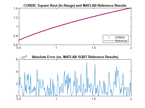
Use the cordicsqrt function to compute the approximate square root of v_fix using ten CORDIC kernel iterations.
step  = 2^-7;
v_fix = fi(0.5:step:(2-step), 1, 20); % fixed-point inputs in range [.5, 2)
niter = 10; % number of CORDIC iterations
x_sqr = cordicsqrt(v_fix, niter);
Get the real-world value (RWV) of the CORDIC outputs for comparison and plot the error between the MATLAB reference and CORDIC square root values.
x_cdc = double(x_sqr); % CORDIC results (scaled by An_hp)
v_ref = double(v_fix); % Reference floating-point input values
x_ref = sqrt(v_ref);   % MATLAB reference floating-point results
figure;
subplot(211);
plot(v_ref, x_cdc, 'r.', v_ref, x_ref, 'b-');
legend('CORDIC', 'Reference', 'Location', 'SouthEast');
title('CORDIC Square Root (In-Range) and MATLAB Reference Results');
subplot(212);
absErr = abs(x_ref - x_cdc);
plot(v_ref, absErr);
title('Absolute Error (vs. MATLAB SQRT Reference Results)');
Overcoming Algorithm Input Range Limitations
Many square root algorithms normalize the input value, , to within the range of [0.5, 2). This pre-processing is typically done using a fixed word length normalization, and can be used to support small as well as large input value ranges.
The CORDIC-based square root algorithm implementation is particularly sensitive to inputs outside of this range. The cordicsqrt function overcomes this algorithm range limitation through a normalization approach based on the following mathematical relationships:
, for some and some even integer .
Thus:
In the cordicsqrt function, the values for and , described above, are found during normalization of the input . is the number of leading zero most-significant bits (MSBs) in the binary representation of the input . These values are found through a series of bit-wise logic and shifts. Note that because must be even, if the number of leading zero MSBs is odd, one additional bit shift is made to make even. The resulting value after these shifts is the value .
becomes the input to the CORDIC-based square root kernel, where an approximation to is calculated. The result is then scaled by so that it is back in the correct output range. This is achieved through a simple bit shift by bits. The (left or right) shift direction depends on the sign of .
Example
Compute the square root of 10-bit fixed-point input data with a small non-negative range using CORDIC. Compare the CORDIC-based algorithm results to the floating-point MATLAB reference results over the same input range.
step     = 2^-8;
u_ref    = 0:step:(0.5-step); % Input array (small range of values)
u_in_arb = fi(u_ref,0,10);    % 10-bit unsigned fixed-point input data values
u_len    = numel(u_ref);
sqrt_ref = sqrt(double(u_in_arb)); % MATLAB sqrt reference results
niter    = 10;
results  = zeros(u_len, 2);
results(:,2) = sqrt_ref(:);
Compute the equivalent real-world value (RWV) result. Plot the RWV of CORDIC and MATLAB reference results.
x_out = cordicsqrt(u_in_arb, niter);
results(:,1) = double(x_out);
figure;
subplot(211);
plot(u_ref, results(:,1), 'r.', u_ref, results(:,2), 'b-');
legend('CORDIC', 'Reference', 'Location', 'SouthEast');
title('CORDIC Square Root (Small Input Range) and MATLAB Reference Results');
axis([0 0.5 0 0.75]);
subplot(212);
absErr = abs(results(:,2) - results(:,1));
plot(u_ref, absErr);
title('Absolute Error (vs. MATLAB SQRT Reference Results)');

Example
Compute the square root of 16-bit fixed-point input data with a large positive range using CORDIC. Compare the CORDIC-based algorithm results to the floating-point MATLAB reference results over the same input range.
u_ref    = 0:5:2500;       % Input array (larger range of values)
u_in_arb = fi(u_ref,0,16); % 16-bit unsigned fixed-point input data values
u_len    = numel(u_ref);
sqrt_ref = sqrt(double(u_in_arb)); % MATLAB sqrt reference results
niter    = 16;
results  = zeros(u_len, 2);
results(:,2) = sqrt_ref(:);
Compute the equivalent real-world value (RWV) result. Plot the RWV of CORDIC and MATLAB reference results.
x_out = cordicsqrt(u_in_arb, niter);
results(:,1) = double(x_out);
figure;
subplot(211);
plot(u_ref, results(:,1), 'r.', u_ref, results(:,2), 'b-');
legend('CORDIC', 'Reference', 'Location', 'SouthEast');
title('CORDIC Square Root (Large Input Range) and MATLAB Reference Results');
axis([0 2500 0 55]);
subplot(212);
absErr = abs(results(:,2) - results(:,1));
plot(u_ref, absErr);
title('Absolute Error (vs. MATLAB SQRT Reference Results)');

References
Jack E. Volder, "The CORDIC Trigonometric Computing Technique," IRE Transactions on Electronic Computers, Volume EC-8, September 1959, pp. 330-334.
J.S. Walther, "A Unified Algorithm for Elementary Functions," Conference Proceedings, Spring Joint Computer Conference, May 1971, pp. 379-385.
See Also
You can also select a web site from the following list:
Americas
- América Latina (Español)
- Canada (English)
- United States (English)
Europe
- Belgium (English)
- Denmark (English)
- Deutschland (Deutsch)
- España (Español)
- Finland (English)
- France (Français)
- Ireland (English)
- Italia (Italiano)
- Luxembourg (English)
- Netherlands (English)
- Norway (English)
- Österreich (Deutsch)
- Portugal (English)
- Sweden (English)
- Switzerland
- United Kingdom (English)