Estimate Position and Orientation of a Ground Vehicle
This example shows how to estimate the position and orientation of ground vehicles by fusing data from an inertial measurement unit (IMU) and a global positioning system (GPS) receiver.
Simulation Setup
Set the sampling rates. In a typical system, the accelerometer and gyroscope in the IMU run at relatively high sample rates. The complexity of processing data from those sensors in the fusion algorithm is relatively low. Conversely, the GPS runs at a relatively low sample rate and the complexity associated with processing it is high. In this fusion algorithm the GPS samples are processed at a low rate, and the accelerometer and gyroscope samples are processed together at the same high rate.
To simulate this configuration, the IMU (accelerometer and gyroscope) is sampled at 100 Hz, and the GPS is sampled at 10 Hz.
imuFs = 100;
gpsFs = 10;

% Define where on the Earth this simulation takes place using latitude,
% longitude, and altitude (LLA) coordinates.
localOrigin = [42.2825 -71.343 53.0352];

% Validate that the |gpsFs| divides |imuFs|. This allows the sensor sample
% rates to be simulated using a nested for loop without complex sample rate
% matching.

imuSamplesPerGPS = (imuFs/gpsFs);
assert(imuSamplesPerGPS == fix(imuSamplesPerGPS), ...
    'GPS sampling rate must be an integer factor of IMU sampling rate.');
Fusion Filter
Create the filter to fuse IMU + GPS measurements. The fusion filter uses an extended Kalman filter to track orientation (as a quaternion), position, velocity, and sensor biases.
The insfilterNonholonomic object has two main methods: predict and fusegps. The predict method takes the accelerometer and gyroscope samples from the IMU as input. Call the predict method each time the accelerometer and gyroscope are sampled. This method predicts the states forward one time step based on the accelerometer and gyroscope. The error covariance of the extended Kalman filter is updated in this step.
The fusegps method takes the GPS samples as input. This method updates the filter states based on the GPS sample by computing a Kalman gain that weights the various sensor inputs according to their uncertainty. An error covariance is also updated in this step, this time using the Kalman gain as well.
The insfilterNonholonomic object has two main properties: IMUSampleRate and DecimationFactor. The ground vehicle has two velocity constraints that assume it does not bounce off the ground or slide on the ground. These constraints are applied using the extended Kalman filter update equations. These updates are applied to the filter states at a rate of IMUSampleRate/DecimationFactor Hz.
gndFusion = insfilterNonholonomic('ReferenceFrame', 'ENU', ...
    'IMUSampleRate', imuFs, ...
    'ReferenceLocation', localOrigin, ...
    'DecimationFactor', 2);
Create Ground Vehicle Trajectory
The waypointTrajectory object calculates pose based on specified sampling rate, waypoints, times of arrival, and orientation. Specify the parameters of a circular trajectory for the ground vehicle.
% Trajectory parameters
r = 8.42; % (m)
speed = 2.50; % (m/s)
center = [0, 0]; % (m)
initialYaw = 90; % (degrees)
numRevs = 2;

% Define angles theta and corresponding times of arrival t.
revTime = 2*pi*r / speed;
theta = (0:pi/2:2*pi*numRevs).';
t = linspace(0, revTime*numRevs, numel(theta)).';

% Define position.
x = r .* cos(theta) + center(1);
y = r .* sin(theta) + center(2);
z = zeros(size(x));
position = [x, y, z];

% Define orientation.
yaw = theta + deg2rad(initialYaw);
yaw = mod(yaw, 2*pi);
pitch = zeros(size(yaw));
roll = zeros(size(yaw));
orientation = quaternion([yaw, pitch, roll], 'euler', ...
    'ZYX', 'frame');

% Generate trajectory.
groundTruth = waypointTrajectory('SampleRate', imuFs, ...
    'Waypoints', position, ...
    'TimeOfArrival', t, ...
    'Orientation', orientation);

% Initialize the random number generator used to simulate sensor noise.
rng('default');
GPS Receiver
Set up the GPS at the specified sample rate and reference location. The other parameters control the nature of the noise in the output signal.
gps = gpsSensor('UpdateRate', gpsFs, 'ReferenceFrame', 'ENU');
gps.ReferenceLocation = localOrigin;
gps.DecayFactor = 0.5;                % Random walk noise parameter
gps.HorizontalPositionAccuracy = 1.0;
gps.VerticalPositionAccuracy =  1.0;
gps.VelocityAccuracy = 0.1;
IMU Sensors
Typically, ground vehicles use a 6-axis IMU sensor for pose estimation. To model an IMU sensor, define an IMU sensor model containing an accelerometer and gyroscope. In a real-world application, the two sensors could come from a single integrated circuit or separate ones. The property values set here are typical for low-cost MEMS sensors.
imu = imuSensor('accel-gyro', ...
    'ReferenceFrame', 'ENU', 'SampleRate', imuFs);

% Accelerometer
imu.Accelerometer.MeasurementRange =  19.6133;
imu.Accelerometer.Resolution = 0.0023928;
imu.Accelerometer.NoiseDensity = 0.0012356;

% Gyroscope
imu.Gyroscope.MeasurementRange = deg2rad(250);
imu.Gyroscope.Resolution = deg2rad(0.0625);
imu.Gyroscope.NoiseDensity = deg2rad(0.025);
Initialize the States of the insfilterNonholonomic
The states are:
States                            Units    Index
Orientation (quaternion parts)             1:4
Gyroscope Bias (XYZ)              rad/s    5:7
Position (NED)                    m        8:10
Velocity (NED)                    m/s      11:13
Accelerometer Bias (XYZ)          m/s^2    14:16
Ground truth is used to help initialize the filter states, so the filter converges to good answers quickly.
% Get the initial ground truth pose from the first sample of the trajectory
% and release the ground truth trajectory to ensure the first sample is not
% skipped during simulation.
[initialPos, initialAtt, initialVel] = groundTruth();
reset(groundTruth);

% Initialize the states of the filter
gndFusion.State(1:4) = compact(initialAtt).';
gndFusion.State(5:7) = imu.Gyroscope.ConstantBias;
gndFusion.State(8:10) = initialPos.';
gndFusion.State(11:13) = initialVel.';
gndFusion.State(14:16) = imu.Accelerometer.ConstantBias;
Initialize the Variances of the insfilterNonholonomic
The measurement noises describe how much noise is corrupting the GPS reading based on the gpsSensor parameters and how much uncertainty is in the vehicle dynamic model.
The process noises describe how well the filter equations describe the state evolution. Process noises are determined empirically using parameter sweeping to jointly optimize position and orientation estimates from the filter.
% Measurement noises
Rvel = gps.VelocityAccuracy.^2;
Rpos = gps.HorizontalPositionAccuracy.^2;

% The dynamic model of the ground vehicle for this filter assumes there is
% no side slip or skid during movement. This means that the velocity is
% constrained to only the forward body axis. The other two velocity axis
% readings are corrected with a zero measurement weighted by the
% |ZeroVelocityConstraintNoise| parameter.
gndFusion.ZeroVelocityConstraintNoise = 1e-2;

% Process noises
gndFusion.GyroscopeNoise = 4e-6;
gndFusion.GyroscopeBiasNoise = 4e-14;
gndFusion.AccelerometerNoise = 4.8e-2;
gndFusion.AccelerometerBiasNoise = 4e-14;

% Initial error covariance
gndFusion.StateCovariance = 1e-9*eye(16);
Initialize Scopes
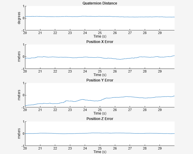
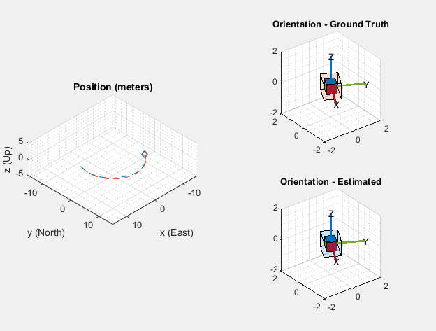
The HelperScrollingPlotter scope enables plotting of variables over time. It is used here to track errors in pose. The HelperPoseViewer scope allows 3-D visualization of the filter estimate and ground truth pose. The scopes can slow the simulation. To disable a scope, set the corresponding logical variable to false.
useErrScope = true; % Turn on the streaming error plot
usePoseView = true;  % Turn on the 3D pose viewer

if useErrScope
    errscope = HelperScrollingPlotter( ...
            'NumInputs', 4, ...
            'TimeSpan', 10, ...
            'SampleRate', imuFs, ...
            'YLabel', {'degrees', ...
            'meters', ...
            'meters', ...
            'meters'}, ...
            'Title', {'Quaternion Distance', ...
            'Position X Error', ...
            'Position Y Error', ...
            'Position Z Error'}, ...
            'YLimits', ...
            [-1, 1
             -1, 1
             -1, 1
             -1, 1]);
end

if usePoseView
    viewer = HelperPoseViewer( ...
        'XPositionLimits', [-15, 15], ...
        'YPositionLimits', [-15, 15], ...
        'ZPositionLimits', [-5, 5], ...
        'ReferenceFrame', 'ENU');
end
Simulation Loop
The main simulation loop is a while loop with a nested for loop. The while loop executes at the gpsFs, which is the GPS measurement rate. The nested for loop executes at the imuFs, which is the IMU sample rate. The scopes are updated at the IMU sample rate.
totalSimTime = 30; % seconds

% Log data for final metric computation.
numGPSSamples = floor(min(t(end), totalSimTime) * gpsFs);
numSamples = numGPSSamples*imuSamplesPerGPS;
truePosition = zeros(numSamples,3);
trueOrientation = quaternion.zeros(numSamples,1);
estPosition = zeros(numSamples,3);
estOrientation = quaternion.zeros(numSamples,1);

idx = 0;

for sampleIdx = 1:numGPSSamples
    % Predict loop at IMU update frequency.
    for i = 1:imuSamplesPerGPS
        if ~isDone(groundTruth)
            idx = idx + 1;

            % Simulate the IMU data from the current pose.
            [truePosition(idx,:), trueOrientation(idx,:), ...
                trueVel, trueAcc, trueAngVel] = groundTruth();
            [accelData, gyroData] = imu(trueAcc, trueAngVel, ...
                trueOrientation(idx,:));

            % Use the predict method to estimate the filter state based
            % on the accelData and gyroData arrays.
            predict(gndFusion, accelData, gyroData);

            % Log the estimated orientation and position.
            [estPosition(idx,:), estOrientation(idx,:)] = pose(gndFusion);

            % Compute the errors and plot.
            if useErrScope
                orientErr = rad2deg( ...
                    dist(estOrientation(idx,:), trueOrientation(idx,:)));
                posErr = estPosition(idx,:) - truePosition(idx,:);
                errscope(orientErr, posErr(1), posErr(2), posErr(3));
            end

            % Update the pose viewer.
            if usePoseView
                viewer(estPosition(idx,:), estOrientation(idx,:), ...
                    truePosition(idx,:), trueOrientation(idx,:));
            end
        end
    end

    if ~isDone(groundTruth)
        % This next step happens at the GPS sample rate.
        % Simulate the GPS output based on the current pose.
        [lla, gpsVel] = gps(truePosition(idx,:), trueVel);

        % Update the filter states based on the GPS data.
        fusegps(gndFusion, lla, Rpos, gpsVel, Rvel);
    end
end
Error Metric Computation
Position and orientation were logged throughout the simulation. Now compute an end-to-end root mean squared error for both position and orientation.
posd = estPosition - truePosition;

% For orientation, quaternion distance is a much better alternative to
% subtracting Euler angles, which have discontinuities. The quaternion
% distance can be computed with the |dist| function, which gives the
% angular difference in orientation in radians. Convert to degrees for
% display in the command window.

quatd = rad2deg(dist(estOrientation, trueOrientation));

% Display RMS errors in the command window.
fprintf('\n\nEnd-to-End Simulation Position RMS Error\n');
End-to-End Simulation Position RMS Error
msep = sqrt(mean(posd.^2));
fprintf('\tX: %.2f , Y: %.2f, Z: %.2f   (meters)\n\n', msep(1), ...
    msep(2), msep(3));
X: 1.16 , Y: 0.98, Z: 0.03 (meters)
fprintf('End-to-End Quaternion Distance RMS Error (degrees) \n');End-to-End Quaternion Distance RMS Error (degrees)
fprintf('\t%.2f (degrees)\n\n', sqrt(mean(quatd.^2)));0.11 (degrees)
Select a Web Site
Choose a web site to get translated content where available and see local events and offers. Based on your location, we recommend that you select: United States.
You can also select a web site from the following list
Americas
- América Latina (Español)
- Canada (English)
- United States (English)
Europe
- Belgium (English)
- Denmark (English)
- Deutschland (Deutsch)
- España (Español)
- Finland (English)
- France (Français)
- Ireland (English)
- Italia (Italiano)
- Luxembourg (English)
- Netherlands (English)
- Norway (English)
- Österreich (Deutsch)
- Portugal (English)
- Sweden (English)
- Switzerland
- United Kingdom (English)
Asia Pacific
- Australia (English)
- India (English)
- New Zealand (English)
- 中国
- 日本Japanese (日本語)
- 한국Korean (한국어)