Multiplatform Radar Detection Fusion
This example shows how to fuse radar detections from a multiplatform radar network. The network includes two airborne and one ground-based long-range radar platforms. See the Multiplatform Radar Detection Generation example for details. A central tracker processes the detections from all platforms at a fixed update interval. This enables you to evaluate the network's performance against target types, platform maneuvers, as well as platform configurations and locations..
Load a recording of a tracking scenario
The MultiplatformRadarDetectionGeneration MAT-file contains a tracking scenario recording previously generated using the following command
recording = record(scene,'IncludeSensors',true,'InitialSeed',2018,'RecordingFormat','Recording')
where scene is the tracking scenario created in the Multiplatform Radar Detection Generation example.
load('MultiplatformScenarioRecording.mat');Define Central Tracker
Use the trackerGNN as a central tracker that processes detections received from all radar platforms in the scenario.
The tracker uses the initFilter supporting function to initialize a constant velocity extended Kalman filter for each new track. initFilter modifies the filter returned by initcvekf to match the high target velocities. The filter's process noise is set to 1 () to enable tracking of maneuvering targets in the scenario.
The tracker's AssignmentThreshold is set to 50 to enable detections with large range biases (due to atmospheric refraction effects at long detection ranges) to be associated with tracks in the tracker. The DeletionThreshold is set to 3 to delete redundant tracks quickly.
Enable the HasDetectableTrackIDsInput to specify the tracks that are within the field of view of at least one radar since the last update. Track logic is only evaluated on tracks which had a detection opportunity since the last tracker update.
tracker = trackerGNN('FilterInitializationFcn', @initFilter, ...
        'AssignmentThreshold', 50, 'DeletionThreshold', 3, ...
        'HasDetectableTrackIDsInput', true);
Track Targets by Fusing Detections in a Central Tracker
The following loop runs the tracking scenario recording until the end of the scenario. For each step forward in the scenario, detections are collected for processing by the central tracker. The tracker is updated with these detections every 2 seconds.
trackUpdateRate = 0.5;   % Update the tracker every 2 seconds

% Create a display to show the true, measured, and tracked positions of the
% detected targets and platforms.
theaterDisplay = helperMultiPlatFusionDisplay(recording,'PlotAssignmentMetrics', true);

% Construct an object to analyze assignment and error metrics
tam = trackAssignmentMetrics('DistanceFunctionFormat','custom',...
    'AssignmentDistanceFcn',@truthAssignmentDistance,...
    'DivergenceDistanceFcn',@truthAssignmentDistance);

% Initialize buffers
detBuffer = {};
sensorConfigBuffer = [];
allTracks = [];
detectableTrackIDs = uint32([]);
assignmentTable = [];

% Initialize next tracker update time
nextTrackUpdateTime = 2;

while ~isDone(recording)
    % Read the next record of the recording.
    [time, truePoses, covcon, dets, senscon, sensPlatIDs] = read(recording);

    % Buffer all detections and sensor configurations until the next tracker update
    detBuffer = [detBuffer ; dets]; %#ok<AGROW>
    sensorConfigBuffer = [sensorConfigBuffer ; senscon']; %#ok<AGROW>

    % Follow the trackUpdateRate to update the tracker
    if time >= nextTrackUpdateTime || isDone(recording)

        if isempty(detBuffer)
            lastDetectionTime = time;
        else
            lastDetectionTime = detBuffer{end}.Time;
        end

        if isLocked(tracker)
            % Collect list of tracks which fell within at least one radar's field
            % of view since the last tracker update
            predictedtracks = predictTracksToTime(tracker, 'all', lastDetectionTime);
            detectableTrackIDs = detectableTracks(allTracks, predictedtracks, sensorConfigBuffer);
        end

        % Update tracker. Only run track logic on tracks that fell within at
        % least one radar's field of view since the last tracker update
        [confirmedTracks, ~, allTracks] = tracker(detBuffer, lastDetectionTime, detectableTrackIDs);

        % Analyze and retrieve the current track-to-truth assignment metrics
        tam(confirmedTracks, truePoses);

        % Store assignment metrics in a table
        currentAssignmentTable = trackMetricsTable(tam);
        rowTimes = seconds(time*ones(size(currentAssignmentTable,1),1));
        assignmentTable = cat(1,assignmentTable,table2timetable(currentAssignmentTable,'RowTimes',rowTimes));

        % Update display with detections, coverages, and tracks
        theaterDisplay(detBuffer, covcon, confirmedTracks, assignmentTable, truePoses, sensPlatIDs);

        % Empty buffers
        detBuffer = {};
        sensorConfigBuffer = [];

        % Update next track update time
        nextTrackUpdateTime = nextTrackUpdateTime + 1/trackUpdateRate;
    end

end
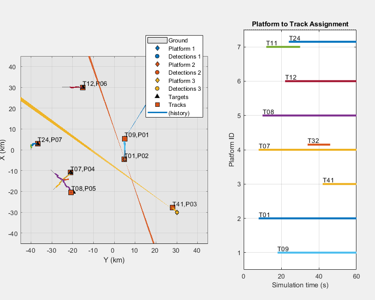
At the end of the scenario, you see that multiple tracks have been dropped and replaced. You can also see the association of tracks to platforms for the duration of the scenario. The plot has seven rows for seven platforms in the scenario. Each track is shown as a horizontal line. Track numbers are annotated at the beginning of the lines. Whenever a track is deleted, its line stops. Whenever a new track is assigned to a platform, a new line is added to the platform's row, when multiple lines are shown at the same time for a single platform, the platform has multiple tracks assigned to it. In these cases, the newer track associated with the platform is considered as redundant.
endTime = assignmentTable.Time(end);
assignmentTable(endTime,{'TrackID','AssignedTruthID','TotalLength','DivergenceCount','RedundancyCount','RedundancyLength'})ans=9×6 timetable
Time TrackID AssignedTruthID TotalLength DivergenceCount RedundancyCount RedundancyLength
______ _______ _______________ ___________ _______________ _______________ ________________
60 sec 1 2 27 0 0 0
60 sec 7 4 27 0 0 0
60 sec 8 5 26 0 0 0
60 sec 9 1 22 0 0 0
60 sec 11 NaN 10 0 0 0
60 sec 12 6 20 0 0 0
60 sec 24 7 19 0 1 4
60 sec 32 NaN 7 0 1 7
60 sec 41 3 10 0 0 0
Notice that the platforms which have difficulties in maintaining tracks (platforms 4 and 7) are also the platforms furthest from the radars. This poor tracking performance is attributed to the Gaussian distribution assumption for the measurement noise. The assumption works well for targets at short ranges, but at long ranges, the measurement uncertainty deviates from a Gaussian distribution. The following figure compares the 1-sigma covariance ellipses corresponding to actual target distribution and the distribution of the target given by a radar sensor. The sensor is 5 km away from the target with an angular resolution of 5 degrees. The actual measurement uncertainty has a concave shape resulting from the spherical sensor detection coordinate frame in which the radar estimates the target's position.
maxCondNum = 300;
figure;
helperPlotLongRangeCorrection(maxCondNum)
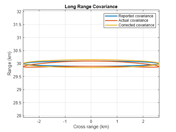
To account for the concave shape of the actual covariance at long ranges, the longRangeCorrection supporting function constrains the condition number of the reported measurement noise. The corrected measurement covariance shown above is constrained to a maximum condition number of 300. In other words, no eigenvalue in the measurement covariance can be more than 300 times smaller than the covariance's largest eigenvalue. This treatment expands the measurement noise along the range dimension to better match the concavity of the actual measurement uncertainty.
Simulate with Long-Range Covariance Correction
Rerun the previous simulation using the longRangeCorrection supporting function to correct the reported measurement noise at long ranges.
[confirmedTracks,correctedAssignmentTable,ctheaterDisplay] = ...
    runMultiPlatFusionSim(recording,tracker,@longRangeCorrection);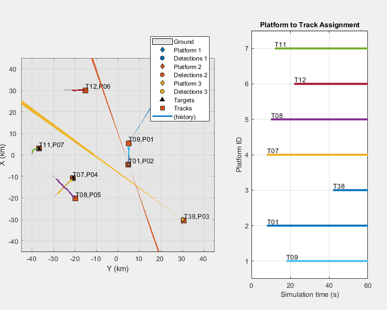
endTime = correctedAssignmentTable.Time(end);
correctedAssignmentTable(endTime,{'TrackID','AssignedTruthID','TotalLength','DivergenceCount','RedundancyCount','RedundancyLength'})ans=7×6 timetable
Time TrackID AssignedTruthID TotalLength DivergenceCount RedundancyCount RedundancyLength
______ _______ _______________ ___________ _______________ _______________ ________________
60 sec 1 2 27 0 0 0
60 sec 7 4 27 0 0 0
60 sec 8 5 26 0 0 0
60 sec 9 1 22 0 0 0
60 sec 11 7 25 0 0 0
60 sec 12 6 20 0 0 0
60 sec 38 3 10 0 0 0
The preceding figure shows that by applying the long-range correction, no track-drops or multiple tracks are generated for the entire scenario. In this case, there is exactly one track for each platform detected by the surveillance network.
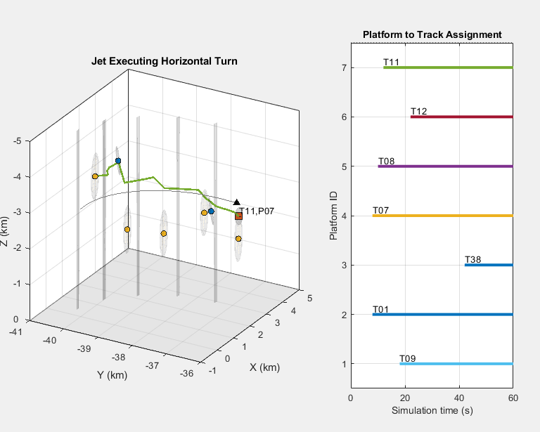
allDetections = vertcat(recording.RecordedData.Detections);
ctheaterDisplay(allDetections,covcon,confirmedTracks,correctedAssignmentTable,truePoses, sensPlatIDs)
axes(ctheaterDisplay.TheaterPlot.Parent)
legend('off')
xlim([-1000 5000]); ylim([-41000 -36000]); zlim([-5000 0]);
view([-90 90])
axis square
title('Jet Executing Horizontal Turn')

Zoom in the view in which the jet is executing a horizontal turn, the track follows the maneuvering target relatively well, even though the motion model used in this example is constant velocity. Tracking the maneuver could be further improved by using an interacting multiple-model (IMM) filter such as the trackingIMM filter.
view([-60 25])
From another view in which the jet is executing a horizontal turn, you can see that the altitude is estimated correctly, despite the inaccurate altitude measurements from the sensors. One of the sensors does not report altitude at all, as seen by the large vertical ellipsoids, while the other two sensors underestimate their uncertainty in the altitude.
xlim([-25000 -9000]); ylim([-31000 -19000]); zlim([-9000 -2000]);
view([-45 10])
title('Crossing Airliners')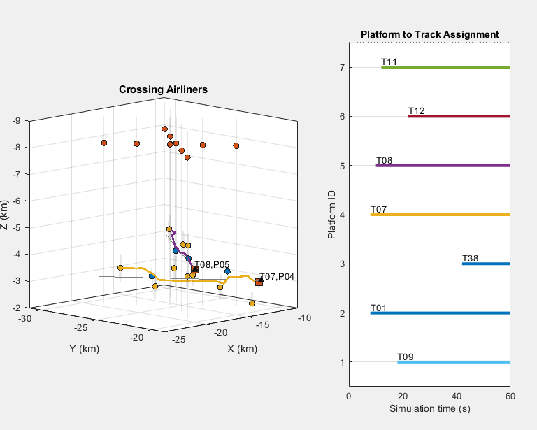
Switching the point of view to focus on the crossing airliners, the same inaccurate altitude measurements are depicted. Note how the red detections are centered at an altitude of 8 km, while the two airliners fly at altitudes of 3 and 4 km, respectively. The use of a very large covariance in the altitude allows the tracker to ignore the erroneous altitude reading from the red detections and keep track of the altitude using the other two radars. Observing the uncertainty covariance of tracks T07 and T08, you can see that they provide a consistent estimate of platforms P04 and P05, respectively.
xlim([-10000 10000]); ylim([-0 10000]); zlim([-12000 -5000]);
view([-15 10])
title('Airborne Radar Platforms')
The last plot focuses on the two airborne radar platforms. Each platform is detected by the other platform as well as by the ground radar. The platform trajectories cross each other, separated by 1000 m in altitude, and their tracks are consistent with the ground truth.
Summary
This example shows how to process detections collected across multiple airborne and ground-based radar platforms in a central tracker. In this example, you learned how the measurement noise at long ranges is not accurately modeled by a Gaussian distribution. The concavity of the 1-sigma ellipse of the measurement noise at these long ranges results in poor tracking performance with dropped tracks and multiple tracks assigned to a single platform. You also learned how to correct the measurement noise for detections at long ranges to improve the continuity of the reported tracks.
Supporting Functions
initFilter: This function modifies the function initcvekf to handle higher velocity targets such as the airliners in the scenario.
function filter = initFilter(detection)
filter = initcvekf(detection);
classToUse = class(filter.StateCovariance);

% Airliners can move at speeds around 900 km/h. The velocity is initialized
% to 0, but will need to be able to quickly adapt to aircraft moving at
% these speeds. Use 900 km/h as 1 standard deviation for the velocity
% noise.
spd = 900*1e3/3600; % m/s
velCov = cast(spd^2,classToUse);
cov = filter.StateCovariance;
cov(2,2) = velCov;
cov(4,4) = velCov;
filter.StateCovariance = cov;

% Set filter's process noise to allow for some horizontal maneuver
scaleAccel = cast(10,classToUse);
Q = blkdiag(scaleAccel^2, scaleAccel^2, 1);
filter.ProcessNoise = Q;
end
detectableTracks: This function returns the IDs for tracks that fell within at least one sensor's field of view. The sensor's field of view and orientation relative to the coordinate frame of the tracks is stored in the array of sensor configuration structs. The configuration structs are returned by the radar sensor and can be used to transform track positions and velocities to the sensor's coordinate frame.
function trackIDs = detectableTracks(tracks,predictedtracks,configs)
% Identify which tracks fell within a sensor's field of view

numTrks = size(tracks,1);
[numsteps, numSensors] = size(configs);
allposTrack = zeros(3,numsteps);
isDetectable = false(numTrks,1);
for iTrk = 1:numTrks
    % Interpolate track positions between current position and predicted
    % positions for each simulation step
    posTrack = tracks(iTrk).State(1:2:end);
    posPreditedTrack = predictedtracks(iTrk).State(1:2:end);
    for iPos = 1:3
        allposTrack(iPos,:) = linspace(posTrack(iPos),posPreditedTrack(iPos),numsteps);
    end
    for iSensor = 1:numSensors
        thisConfig = configs(:,iSensor);
        for k = 1:numsteps
            if thisConfig(k).IsValidTime
                pos = trackToSensor(allposTrack(:,k),thisConfig(k));
                % Check if predicted track position is in sensor field of
                % view
                [az,el] = cart2sph(pos(1),pos(2),pos(3));
                az = az*180/pi;
                el = el*180/pi;
                inFov = abs(az)<thisConfig(k).FieldOfView(1)/2 && abs(el) < thisConfig(k).FieldOfView(2)/2;
                if inFov
                    isDetectable(iTrk) = inFov;
                    k = numsteps; %#ok<FXSET>
                    iSensor = numSensors; %#ok<FXSET>
                end
            end
        end
    end

end

trackIDs = [tracks.TrackID]';
trackIDs = trackIDs(isDetectable);
end
trackToSensor: This function returns the track's position in the sensor's coordinate frame. The track structure is returned by the trackerGNN object and the config structure defining the sensor's orientation relative to the track's coordinate frame is returned by the radar object.
function pos = trackToSensor(pos,config)

frames = config.MeasurementParameters;
for m = numel(frames):-1:1
    rotmat = frames(m).Orientation;
    if ~frames(m).IsParentToChild
        rotmat = rotmat';
    end
    offset = frames(m).OriginPosition;
    pos = bsxfun(@minus,pos,offset);
    pos = rotmat*pos;
end
end
longRangeCorrection: This function limits the measurement noise accuracy reported by the radar to not exceed a maximum condition number. The condition number is defined as the ratio of the eigenvalues of the measurement noise to the largest eigenvalue.
When targets are detected at long ranges from a radar, the surface curvature of the uncertainty of the measurement is no longer well approximated by an ellipsoid but takes on that of a concave ellipsoid. The measurement noise must be increased along the range dimension to account for the concavity, producing a planar ellipse which encompasses the concave ellipsoid. There are several techniques in the literature to address this. Here, the maximum condition number of the measurement noise is limited by increasing the smallest eigenvalues to satisfy the maximum condition number constraint. This has the effect of increasing the uncertainty along the range dimension, producing an ellipse which better encloses the concave uncertainty.
function dets = longRangeCorrection(dets,maxCond)
for m = 1:numel(dets)
    R = dets{m}.MeasurementNoise;
    [Q,D] = eig(R);
    Q = real(Q);
    d = real(diag(D));
    dMax = max(d);
    condNums = dMax./d;
    iFix = condNums>maxCond;
    d(iFix) = dMax/maxCond;
    R = Q*diag(d)*Q';
    dets{m}.MeasurementNoise = R;
end
end