Drape Data on Elevation Maps
Combine Elevation Maps with Other Kinds of Data
Lighting effects can provide important visual cues when elevation maps are combined with other kinds of data. The shading resulting from lighting a surface makes it possible to "drape" satellite data over a grid of elevations. It is common to use this kind of display to overlay georeferenced land cover images from Earth satellites such as LANDSAT and SPOT on topography from digital elevation models.
When the elevation and image data grids correspond pixel-for-pixel to the same geographic locations, you can build up such displays using the optional altitude arguments in the surface display functions. If they do not, you can interpolate one or both source grids to a common mesh.
Drape Data over Terrain with Different Gridding
If you want to combine elevation and attribute (color) data grids that cover the same region but are gridded differently, you must resample one matrix to be consistent with the other. That is, you can construct a geolocated grid version of the regular data grid values or construct a regular grid version of the geolocated data grid values.
It helps if at least one of the grids is a geolocated data grid, because their
explicit horizontal coordinates allow them to be resampled using the
geointerp function. These examples show how to drape data
over terrain with different gridding.
Combine Dissimilar Grids by Converting Regular Grid to Geolocated Data Grid
This example shows how to combine an elevation data grid and an attribute (color) data grid that cover the same region but are gridded differently. The example drapes slope data from a regular data grid on top of elevation data from a geolocated data grid. The example uses the geolocated data grid as the source for surface elevations and transforms the regular data grid into slope values, which are then sampled to conform to the geolocated data grid (creating a set of slope values for the diamond-shaped grid) and color-coded for surface display. This approach works with any dissimilar grids, although the two data sets in this example actually have the same origin (the geolocated grid derives from the topo60c data set).
Load the geolocated data grid from the mapmtx file and the regular data grid from the topo60c file. The mapmtx file actually contains two regions but this example only uses the diamond-shaped portion, lt1, lg1, and map1, centered on the Middle East.
load mapmtx lt1 lg1 map1
load topo60c
Compute the surface aspect, slope, and gradients for topo60c. This example only uses the slopes in subsequent steps.
[aspect,slope,gradN,gradE] = gradientm(topo60c,topo60cR);
Use the geointerp function to interpolate slope values to the geolocated grid specified by lt1 and lg1. The output is a 50-by-50 grid of elevations matching the coverage of the map1 variable.
slope1 = geointerp(slope,topo60cR,lt1,lg1);
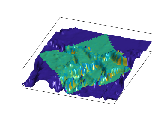
Set up a figure with a Miller projection and use surfm to display the slope data. Specify the z -values for the surface explicitly as the map1 data, which is terrain elevation. The map mainly depicts steep cliffs, which represent mountains (the Himalayas in the northeast), and continental shelves and trenches.
figure
axesm miller
surfm(lt1,lg1,slope1,map1)
The coloration depicts steepness of slope. Change the colormap to make the steepest slopes magenta, the gentler slopes dark blue, and the flat areas light blue:
colormap cool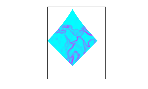
Use view to get a southeast perspective of the surface from a low viewpoint. In 3-D, you can see the topography as well as the slope.
view(20,30)
daspectm('meter',200)
The default rendering uses faceted shading (no smooth interpolation). Make the surface shiny with Gouraud shading and specify lighting from the east (the default of camlight lights surfaces from over the right shoulder of the viewer).
material shiny
camlight
lighting Gouraud
Remove the white space and view the figure in perspective mode.
axis tight
ax = gca;
ax.Projection = 'perspective';
Drape Geolocated Grid on Regular Data Grid via Texture Mapping
This example shows how to create a new regular data grid that covers the region of the geolocated data grid, then embed the color data values into the new matrix. The new matrix might need to have somewhat lower resolution than the original, to ensure that every cell in the new map receives a value. The example combines dissimilar data grids by creating a new regular data grid that covers the region of the geolocated data grid's z-data. This approach has the advantage that more computational functions are available for regular data grids than for geolocated ones. Color and elevation grids do not have to be the same size. If the resolutions of the two data grids are different, you can create the surface as a three-dimensional elevation map and later apply the colors as a texture map. You do this by setting the surface CData property to contain the color matrix, and setting the surface face color to 'texturemap'.
Load elevation raster data and a geographic cells reference object from topo60c.mat. Get individual variables containing terrain data from mapmtx.mat.
load topo60c
load mapmtx lt1 lg1 map1
Identify the geographic limits of the geolocated grid that was loaded from mapmtx.
latlim(1) = 2*floor(min(lt1(:))/2);
lonlim(1) = 2*floor(min(lg1(:))/2);
latlim(2) = 2*ceil(max(lt1(:))/2);
lonlim(2) = 2*ceil(max(lg1(:))/2);
Crop the global elevation data to the rectangular region enclosing the smaller grid.
[topo1,topo1R] = geocrop(topo60c,topo60cR,latlim,lonlim);
Allocate a regular grid filled uniformly with -Inf, to receive texture data.
L1R = georefcells(latlim,lonlim,2,2);
L1 = zeros(L1R.RasterSize);
L1 = L1 - Inf;
Overwrite L1 using imbedm, converting it from a geolocated grid to a regular grid, in which the values come from the discrete Laplacian of the elevation grid map1.
L1 = imbedm(lt1,lg1,del2(map1),L1,L1R);
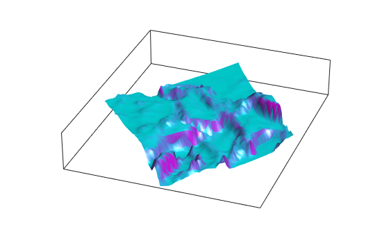
Set up an axesm-based map with the Miller projection and use meshm to display the cropped data. Render the figure as a 3-D view from a 20 degree azimuth and 30 degree altitude, and exaggerate the vertical dimension by a factor of 200. Both the surface relief and coloring represent topographic elevation.
figure
axesm miller
h = meshm(topo1,topo1R,size(topo1),topo1);
view(20,30)
daspectm('m',200)
Apply the L1 matrix as a texture map directly to the surface using the set function. The area not covered by the [lt1,lg1,map1] geolocated data grid appears dark blue because the corresponding elements of L1 were set to -Inf.
h.CData = L1;
h.FaceColor = 'texturemap';
material shiny
camlight
lighting gouraud
axis tight