How Image Data Relates to a Colormap

When you display images using the image function, you can control how the range of pixel values maps to the range of the colormap. For example, here is a 5-by-5 magic square displayed as an image using the default colormap.

A = magic(5) 

A = 5×5

    17    24     1     8    15
    23     5     7    14    16
     4     6    13    20    22
    10    12    19    21     3
    11    18    25     2     9

im = image(A);
axis off
colorbar

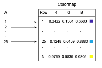
A contains values between 1 and 25. MATLAB^® treats those values as indices into the colormap, which has 64 entries. Thus, all the pixels in the preceding image map to the first 25 entries in the colormap (roughly the blue region of the colorbar).

You can control this mapping with the CDataMapping property of the Image object. The default behavior shown in the preceding diagram corresponds to the 'direct' option for this property. Direct mapping is useful when you are displaying images (such as GIF images) that contain their own colormap. However, if your image represents measurements of some physical unit (e.g., meters or degrees) then set the CDataMapping property to 'scaled'. Scaled mapping uses the full range of colors, and it allows you to visualize the relative differences in your data.

im.CDataMapping = 'scaled';

The 'scaled' option maps the smallest value in A to the first entry in the colormap, and maps largest value in A maps to the last entry in the colormap. All intermediate values of A are linearly scaled to the colormap.

As an alternative to setting the CDataMapping property to 'scaled', you can call the imagesc function to get the same effect.

imagesc(A);
axis off
colorbar

If you change the colormap, the values in A are scaled to the new colormap.

colormap(gray);

Scaled mapping is also useful for displaying pictorial images that have no colormap, or when you want to change the colormap for a pictorial image. The following commands display an image using the gray colormap, which is different than the original colormap that is stored with this image.

load clown
image(X,'CDataMapping','scaled');
colormap(gray);
axis off
colorbar