Nonnegative ODE Solution
This topic shows how to constrain the solution of an ODE to be nonnegative. Imposing nonnegativity is not always trivial, but sometimes it is necessary due to the physical interpretation of the equations or due to the nature of the solution. You should only impose this constraint on the solution when necessary, such as in cases where the integration fails without it, or where the solution would be inapplicable.
If certain components of the solution must be nonnegative, then use odeset to set the NonNegative option for the indices of these components. This option is not available for ode23s, ode15i, or for implicit solvers (ode15s, ode23t, ode23tb) applied to problems with a mass matrix. In particular, you cannot impose nonnegativity constraints on a DAE problem, which necessarily has a singular mass matrix.
Example: Absolute Value Function
Consider the initial value problem
solved on the interval with the initial condition . The solution of this ODE decays to zero. If the solver produces a negative solution value, then it begins to track the solution of the ODE through this value, and the computation eventually fails as the calculated solution diverges to . Using the NonNegative option prevents this integration failure.
Compare the analytic solution of to a solution of the ODE using ode45 with no extra options, and to one with the NonNegative option set.
ode = @(t,y) -abs(y);

% Standard solution with |ode45|
options1 = odeset('Refine',1);
[t0,y0] = ode45(ode,[0 40],1,options1);

% Solution with nonnegative constraint
options2 = odeset(options1,'NonNegative',1);
[t1,y1] = ode45(ode,[0 40],1,options2);

% Analytic solution
t = linspace(0,40,1000);
y = exp(-t);
Plot the three solutions for comparison. Imposing nonnegativity is crucial to keep the solution from veering off toward .
plot(t,y,'b-',t0,y0,'ro',t1,y1,'k*');
legend('Exact solution','No constraints','Nonnegativity', ...
       'Location','SouthWest')

Example: The Knee Problem
Another example of a problem that requires a nonnegative solution is the knee problem coded in the example file kneeode. The equation is
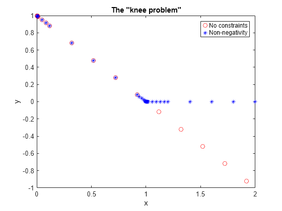
solved on the interval with the initial condition . The parameter generally is taken to satisfy , and this problem uses . The solution to this ODE approaches for and for . However, computing the numerical solution with default tolerances shows that the solution follows the isocline for the whole interval of integration. Imposing nonnegativity constraints results in the correct solution.
Solve the knee problem with and without nonnegativity constraints.
epsilon = 1e-6;
y0 = 1;
xspan = [0 2];
odefcn = @(x,y,epsilon) ((1-x)*y - y^2)/epsilon;

% Solve without imposing constraints
[x1,y1] = ode15s(@(x,y) odefcn(x,y,epsilon), xspan, y0);

% Impose a nonnegativity constraint
options = odeset('NonNegative',1);
[x2,y2] = ode15s(@(x,y) odefcn(x,y,epsilon), xspan, y0, options);
Plot the solutions for comparison.
plot(x1,y1,'ro',x2,y2,'b*')
axis([0,2,-1,1])
title('The "knee problem"')
legend('No constraints','Non-negativity')
xlabel('x')
ylabel('y')

References
[1] Shampine, L.F., S. Thompson, J.A. Kierzenka, and G.D. Byrne, "Non-negative solutions of ODEs," Applied Mathematics and Computation Vol. 170, 2005, pp. 556-569.