Design Model Predictive Controller at Equilibrium Operating Point
This example shows how to design a model predictive controller with nonzero nominal values.
The plant model is obtained by linearization of a nonlinear plant in Simulink® at a nonzero steady-state operating point.
Linearize Nonlinear Plant Model
The nonlinear plant is implemented in the Simulink model mpc_nloffsets and linearized at the default operating condition using the linearize function from Simulink Control Design™.
Create an operating point specification for the current model initial conditions.
plant_mdl = 'mpc_nloffsets';
op = operspec(plant_mdl);
Compute the operating point for these initial conditions.
[op_point, op_report] = findop(plant_mdl,op);
 Operating point search report:
---------------------------------

opreport =


 Operating point search report for the Model mpc_nloffsets.
 (Time-Varying Components Evaluated at time t=0)

Operating point search completed successfully using optimization.
States:
----------
    Min          x          Max        dxMin        dx         dxMax
___________ ___________ ___________ ___________ ___________ ___________

(1.) mpc_nloffsets/Integrator
   -Inf       0.57514       Inf          0      -1.8208e-14      0
(2.) mpc_nloffsets/Integrator2
   -Inf       2.1503        Inf          0      -8.3844e-12      0

Inputs:
----------
 Min     u     Max
______ ______ ______

(1.) mpc_nloffsets/In1
 -Inf  -1.252  Inf

Outputs:
----------
  Min       y       Max
________ ________ ________

(1.) mpc_nloffsets/Out1
  -Inf   -0.52938   Inf
Extract nominal state, output, and input values from the computed operating point.
x0 = [op_report.States(1).x;op_report.States(2).x];
y0 = op_report.Outputs.y;
u0 = op_report.Inputs.u;
Linearize the plant at the initial conditions.
plant = linearize(plant_mdl,op_point);
Design MPC Controller
Create an MPC controller object with a specified sample time Ts, prediction horizon 20, and control horizon 3.
Ts = 0.1;
mpcobj = mpc(plant,Ts,20,3);
-->"Weights.ManipulatedVariables" is empty. Assuming default 0.00000.
-->"Weights.ManipulatedVariablesRate" is empty. Assuming default 0.10000.
-->"Weights.OutputVariables" is empty. Assuming default 1.00000.
Set the nominal values in the controller.
mpcobj.Model.Nominal = struct('X',x0,'U',u0,'Y',y0);
Set the output measurement noise model (white noise, zero mean, standard deviation = 0.1).
mpcobj.Model.Noise = 0.1;
Set the manipulated variable constraint.
mpcobj.MV.Max = 0.2;
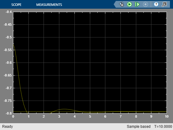
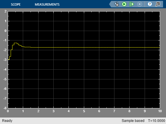
Simulate Using Simulink
Specify the reference value for the output signal.
r0 = 1.5*y0;
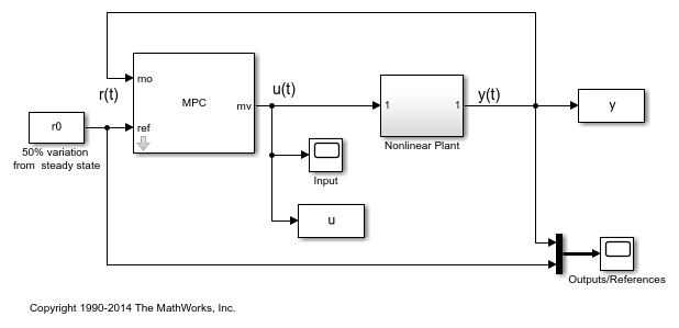
Open and simulate the model.
mdl = 'mpc_offsets';
open_system(mdl)
sim(mdl)
-->Converting model to discrete time.
-->Integrator added as output disturbance model for measured output #1.
Simulate Using sim Command
Simulate the controller.
Tf = round(10/Ts);
r = r0*ones(Tf,1);
[y1,t1,u1,x1,xmpc1] = sim(mpcobj,Tf,r);
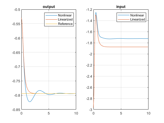
Plot and compare the simulation results.
subplot(1,2,1)
plot(y.time,y.signals.values,t1,y1,t1,r)
legend('Nonlinear','Linearized','Reference')
title('output')
grid

subplot(1,2,2)
plot(u.time,u.signals.values,t1,u1)
legend('Nonlinear','Linearized')
title('input')
grid
bdclose(plant_mdl)
bdclose(mdl)
