Boost Power Train Operating Point Analysis
This example shows how to analyze the operating point of a power train for a boost switched-mode power supply (SMPS) using behavioral circuit modeling and analysis tools from the Mixed-Signal Blockset™.
One of the first steps in the design of a SMPS is to determine the control duty cycle needed to obtain a desired steady state output under a fixed set of supply and load conditions, referred to as an operating point. This analysis must also create the power train small signal control model needed to design the power supply control loop.
Even before the control loop is designed, some form of operating point analysis is needed to choose the power train circuit topology and the circuit elements to be used in the power train. There are typically many options available, and each combination of options that can produce the required output must be analyzed for efficiency, output ripple, input ripple and cost in order to settle on a power train circuit design.
You can use the cktoperpoint to perform a complete operating point analysis, leading to a detailed power train circuit design and the models needed to design the power supply control loop. The design of the power supply control loop is demonstrated in a separate example, Feedback Amplifier Design for Voltage-Mode Boost Converter.
Power Train Circuit
The power train circuit design used in this example was adapted from a widely used tutorial on feedback loop analysis. Operating point analysis must be capable of providing comprehensive information on very detailed circuit designs, and so the circuit design used in this example includes detailed models of commercially available parts for the switching device, diode and inductor (except that the inductance is the 75uH of the original example instead of the 104uH for the commercial part). A load current source is included to model the powering of semiconductor devices.
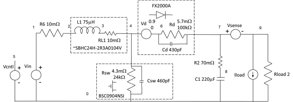
Two resistance values are shown for the switching device and the diode - an "on" resistance and an "off" resistance.
The circuit is described by the Simscape™ model TIBoostPowerTrain.slx. The port controlling the gate of Q1 is implemented by the Controlled Voltage Source cQ1. The prefix "c" differentiates it as a control signal (which can only be 1 or 0), while the "Q1" associates it with transistor Q1. The Equivalent Series Resistance (ESR) of the inductor is modeled by RL1 because the behavioral model ignores the Series resistance parameter from the inductor itself.
modelName = "TIBoostPowerTrain";
load_system(modelName);
Analysis of a Single Design Point
The analysis process begins by configuring the analysis of a single set of circuit element values and operating conditions, referred to in this example as a "design point".
Once the analysis has been configured, you can run the analysis using cktoperpoint. This creates a plot of the selected output as a function of control input, along with a struct containing a table of DC results, a set of detailed waveforms, and the control system matrices needed to construct a small signal model of the power train for use in designing the power supply control loop.
Configuration
Call the cktconfig function to parse the diagram and create a circuit configuration.
Text to display on the block: the model name (TIBoostPowerTrain)
Block name in Simulink: Boost
Port order: cQ1, Vg, Iload, Vout, Iout, Ig
Input values at which to do the analysis: Vin = 10 V, ILoad = 0 A
cfg = cktconfig(modelName, ...
    CircuitDesignName=modelName, ...
    BlockName='Boost', ...
    Ports={'cQ1','Vg','Iload','Vout','Iout','Ig'}, ...
    InputValues={ ...
    'Vg','Iload'; ... % Row 1: Names
    10,   0});         % Row 2: Values);
In addition to the circuit itself, AC operating point analysis requires the following metadata:
Output port to analyze: Vout
Output value(s) to find a duty cycle for: 14 V, 18 V, 24 V
Control variable type: Duty Cycle
Duty cycle range: 10% <= dc <= 90%
Frequency of the control signal: 200 kHz
Phase: 0
Pulse duration variable name: d
Samples per switch cycle: 1024
cfg.OutputPort = 'Vout';
cfg.OutputValues = [14,18,24];
cfg.ControlVariable = 'Duty cycle';
cfg.DutyCycle = [0.1 0.9];
cfg.Frequency = 200000;
cfg.PhaseOffsets = '0';
cfg.PulseDuration = 'd';
cfg.WaveSamples = 1024;

[results,plotdata,waves,ssmodels] = cktoperpoint(cfg);
Results Table
results
results =

  3×7 table

    Duty Cycle    Frequency    Vg    Iload    Vout    Iout      Ig
    __________    _________    __    _____    ____    ____    ______

     0.33461        2e+05      10      0       14     1.4     2.1042
     0.47864        2e+05      10      0       18     1.8     3.4528
     0.60859        2e+05      10      0       24     2.4      6.132
Waveforms
waves{2}(1:10,:)
ans =

  10×23 table

       Time        Vout     Iout_out    Ig_out    State     Iout       Ig       iL1        iVg      icQ1      V1         V2        V3        V4       V5      V6       V7       V8      V9      vdDiode      ivfDiode     vdQ1    ivbdQ1
    __________    ______    ________    ______    _____    ______    ______    ______    _______    ____    ______    ________    _____    ______    _____    __    ________    __    ______    ________    __________    ____    _______

             0    17.884     1.7884     3.2952      3      1.7884    3.2952    3.2952    -3.2952     0       18.01    0.014169    9.967    17.884    9.967    1     0.047122    10    17.884    0.014169    -1.787e-07     0      -3.2952
    4.8828e-09    17.884     1.7884     3.2959      3      1.7884    3.2959    3.2959    -3.2959     0      18.009    0.014172    9.967    17.884    9.967    1     0.047131    10    17.884    0.014172    -1.787e-07     0      -3.2959
    9.7656e-09    17.884     1.7884     3.2965      3      1.7884    3.2965    3.2965    -3.2965     0      18.009    0.014175    9.967    17.884    9.967    1      0.04714    10    17.884    0.014175    -1.787e-07     0      -3.2965
    1.4648e-08    17.884     1.7884     3.2972      3      1.7884    3.2972    3.2972    -3.2972     0      18.009    0.014178    9.967    17.884    9.967    1     0.047149    10    17.884    0.014178    -1.787e-07     0      -3.2972
    1.9531e-08    17.884     1.7884     3.2978      3      1.7884    3.2978    3.2978    -3.2978     0      18.009    0.014181    9.967    17.884    9.967    1     0.047159    10    17.884    0.014181    -1.787e-07     0      -3.2978
    2.4414e-08    17.884     1.7884     3.2984      3      1.7884    3.2984    3.2984    -3.2984     0      18.009    0.014183    9.967    17.884    9.967    1     0.047168    10    17.884    0.014183    -1.787e-07     0      -3.2984
    2.9297e-08    17.884     1.7884     3.2991      3      1.7884    3.2991    3.2991    -3.2991     0      18.009    0.014186    9.967    17.884    9.967    1     0.047177    10    17.884    0.014186    -1.787e-07     0      -3.2991
     3.418e-08    17.884     1.7884     3.2997      3      1.7884    3.2997    3.2997    -3.2997     0      18.009    0.014189    9.967    17.884    9.967    1     0.047186    10    17.884    0.014189    -1.787e-07     0      -3.2997
    3.9063e-08    17.884     1.7884     3.3004      3      1.7884    3.3004    3.3004    -3.3004     0      18.009    0.014192    9.967    17.884    9.967    1     0.047195    10    17.884    0.014192    -1.787e-07     0      -3.3004
    4.3945e-08    17.884     1.7884      3.301      3      1.7884     3.301     3.301     -3.301     0      18.009    0.014194    9.967    17.884    9.967    1     0.047205    10    17.884    0.014194    -1.787e-07     0       -3.301
The waves continue for 1024 samples. Also note that the state and all of the node values are included in the table.
Small Signal Model
ssmodels(:,:,2)
ans =

  A =
            x1       x2
   x1   0.9957  -0.0344
   x2  0.01173   0.9975

  B =
               Vg       Iload  Duty cycle
   x1     0.06657    0.002615       1.267
   x2   0.0002042    -0.02253    -0.07426

  C =
                x1         x2
   Vout    0.03922     0.9918
   Iout   0.003922    0.09918
   Ig       0.9989  -0.008984

  D =
                 Vg       Iload  Duty cycle
   Vout           0    -0.06951           0
   Iout           0       0.993           0
   Ig             0           0           0

Sample time: 5e-06 seconds
Discrete-time state-space model.
Adding Metrics to the Analysis
Given the waveforms in the output struct you can implement your own metrics. The script getPowerTrainMetrics included with this example demonstrates the type of analyses that are possible. This script appends results to the DcResults table show above. It uses the function getCircuitElementPower to perform much of the detailed data access.
Run the getPowerTrainMetrics script, display the power analysis table, the efficiency metrics derived from the power analysis table, and the ripple metrics derived from the waveforms.
results = getPowerTrainMetrics(cfg,waves,results,"V8","Ig","V9","Iout");
Power Analysis Table
results(:,7:18)
ans =

  3×12 table

      Ig       P_Vg      P_Iload      P_R2       P_RL1        P_Rg      P_Rload    P_total    Efficiency    Vin_ripple    Iin_ripple    Vout_ripple
    ______    _______    _______    ________    ________    ________    _______    _______    __________    __________    __________    ___________

    2.1042    -21.049       0       0.068268    0.044345    0.044345      19.6     -1.2912     0.93317          0          0.22182          0.154
    3.4528    -34.534       0        0.20571     0.11934     0.11934    32.401     -1.6892     0.94147          0          0.31633        0.25104
     6.132    -61.327       0        0.61808     0.37623     0.37623    57.602     -2.3541     0.94506          0          0.39955        0.44511
Efficiency and Ripple Metrics
results(:,19:end)
ans =

  3×1 table

    Iout_ripple
    ___________

       0.0154
     0.025104
     0.044511