Reconstruct Phase Space and Estimate Condition Indicators Using Live Editor Tasks
This example shows how use Live Editor tasks to reconstruct phase space of a uniformly sampled signal and then use the reconstructed phase space to estimate the correlation dimension and the Lyapunov exponent.
Live Editor tasks let you interactively iterate on parameters and settings while observing their effects on the result of your computation. The tasks then and automatically generate MATLAB® code that achieves the displayed results. To experiment with the Live Editor tasks in this script, open this example.
For more information about Live Editor Tasks generally, see Add Interactive Tasks to a Live Script.
Load Data
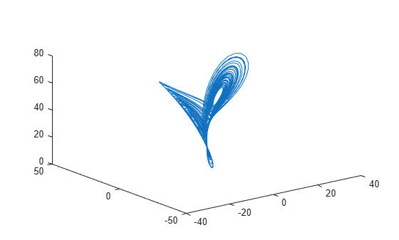
In this example, assume that you have measurements for a Lorenz Attractor. Your measurements are along the x-direction only, but the attractor is a three-dimensional system. Using this limited data, reconstruct the phase space such that the properties of the original three-dimensional system are recovered.
Load the Lorenz Attractor data, and visualize its x, y and z measurements on a 3-D plot. Since the Lorenz attractor has 3 dimensions, specify dim as 3.
load('lorenzAttractorExampleData.mat','data','fs')
X = data(:,1);
plot3(data(:,1),data(:,2),data(:,3));
Reconstruct Phase Space
To reconstruct the phase space data, use the Reconstruct Phase Space Live Editor Task. You can insert a task into your script using the Task menu in the Live Editor. In this script, Reconstruct Phase Space is already inserted. Open the example to experiment with the task.
To perform the phase space reconstruction, in the task, specify the signal you loaded, X and the embedding dimension as 3. In the Reconstruct Phase Space task, you can experiment with different lag and embedding dimension values and observe the reconstructed Lorenz attractor displayed in the output plot. For details about the available options and parameters, see the Reconstruct Phase Space task reference page.

After you finish experimenting with the task, the reconstructed phase space data phaseSpace and the estimated time delay lag are in the MATLAB® workspace, and you can use them to identify different condition indicators for the Lorenz attractor. For instance, estimate the correlation dimension and the Lyapunov exponent values using phaseSpace.
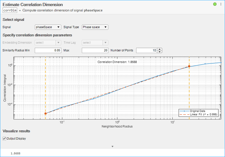
Estimate Correlation Dimension
To estimate the correlation dimension, use the Estimate Correlation Dimension Live Editor Task. In the task, specify the phase space signal, phaseSpace from the workspace. Specify signal type as Phase space. The task automatically computes the embedding dimension and lag values from the phase space signal. For this example, use 0.05 and 20 for the minimum and maximum similarity radius values and the default value of 10 points. In the Estimate Correlation Dimension task, you can experiment with similarity radius values and number of points to align the linear fit line with the original correlation integral data line in the output plot. For details about the available options and parameters, see the Estimate Correlation Dimension task reference page.
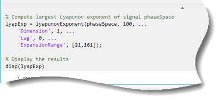
As you vary parameters in the task, it automatically updates the generated code for performing the estimation and creating the plot. (To see the generated code, click ![]() at the bottom of the task.)
at the bottom of the task.)
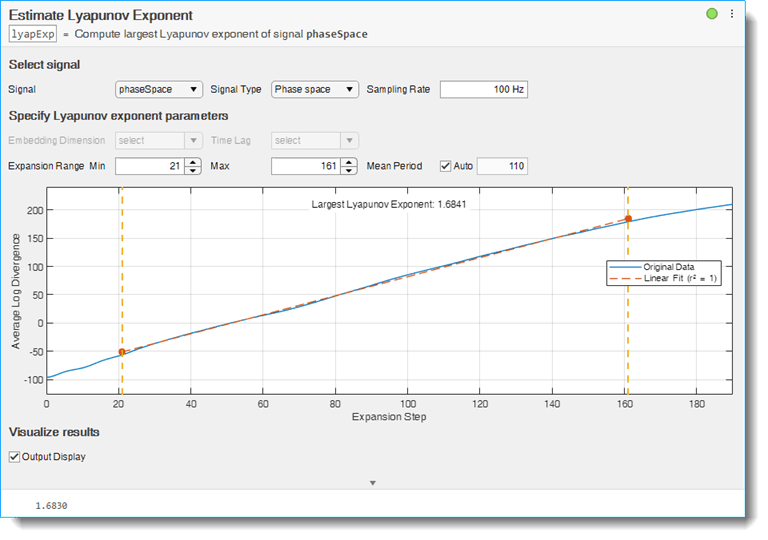
Estimate Lyapunov Exponent
To estimate the Lyapunov Exponent, use the Estimate Lyapunov Exponent Live Editor Task. In the task, specify the phase space signal, phaseSpace from the workspace. Specify signal type as Phase space and the sampling rate as 100 Hz. The task automatically computes the embedding dimension and lag values from the phase space signal. For this example, use 21 and 161 for the minimum and maximum expansion range values and the default value of 110 for the mean period. In the Estimate Lyapunov Exponent task, you can experiment with expansion range and mean period values to align the linear fit line with the original log divergence data line in the output plot. For details about the available options and parameters, see the Estimate Lyapunov Exponent task reference page.
Generate Code
As you vary parameters in each task, it automatically updates the generated code for performing the estimation and creating the plot. To see the generated code, click ![]() at the bottom of the task. You can cut and paste this code to use or modify later in the existing script or a different program. For example:
at the bottom of the task. You can cut and paste this code to use or modify later in the existing script or a different program. For example:
Because the underlying code is now part of your live script, you can continue to use the variables created by each task for further processing.
See Also
Reconstruct
Phase Space | Estimate
Approximate Entropy | Estimate
Correlation Dimension | Estimate
Lyapunov Exponent | approximateEntropy | correlationDimension | lyapunovExponent | phaseSpaceReconstruction