Main Content

Interdigital Capacitor - Visualize and Analyze

This example shows you how to create, visualize, and analyze an interdigital capacitor.

Create an interdigital capacitor with default properties.

capacitor = interdigitalCapacitor
capacitor = 
  interdigitalCapacitor with properties:

            NumFingers: 4
          FingerLength: 0.0137
           FingerWidth: 3.1600e-04
         FingerSpacing: 3.0000e-04
         FingerEdgeGap: 3.4100e-04
    TerminalStripWidth: 5.0000e-04
         PortLineWidth: 0.0019
        PortLineLength: 0.0030
                Height: 7.8700e-04
      GroundPlaneWidth: 0.0030
             Substrate: [1x1 dielectric]
             Conductor: [1x1 metal]
            SolverType: 'MoM'
            IsShielded: 0

View the capacitor.

show(capacitor)
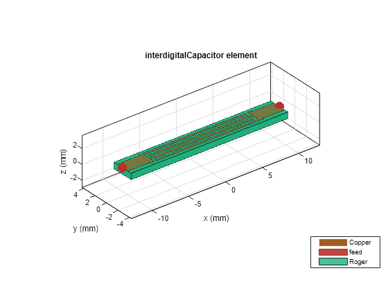
Figure contains an axes object. The axes object with title interdigitalCapacitor element, xlabel x (mm), ylabel y (mm) contains 6 objects of type patch, surface. These objects represent Copper, feed, Roger.

Plot the charge distribution at 5 GHz.

charge(capacitor, 5e9)

Figure contains an axes object. The axes object with title Charge distribution, xlabel x (m), ylabel y (m) contains 4 objects of type patch.

Plot the current distribution at 5 GHz.

figure
current(capacitor, 5e9)
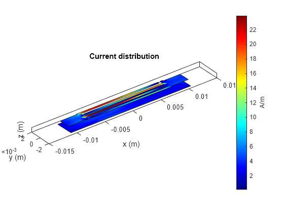
Figure contains an axes object. The axes object with title Current distribution, xlabel x (m), ylabel y (m) contains 4 objects of type patch.

Calculate and plot the s-parameters.

spar = sparameters(capacitor,linspace(1e9,10e9,30));
rfplot(spar)
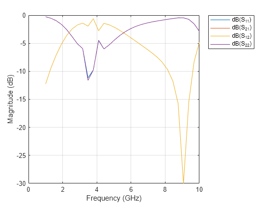
Figure contains an axes object. The axes object with xlabel Frequency (GHz), ylabel Magnitude (dB) contains 4 objects of type line. These objects represent dB(S_{11}), dB(S_{21}), dB(S_{12}), dB(S_{22}).