Main Content

Shunt Radial Stub - Visualize and Analyze

This example shows you how to create, visualize, and analyze a radial stub shunt on the X-Y plane.

Create a shunt radial stub with default properties.

stub = stubRadialShunt
stub = 
  stubRadialShunt with properties:

             StubType: 'Single'
          OuterRadius: 0.0085
          InnerRadius: 0.0012
                Angle: 90
       PortLineLength: 0.0137
        PortLineWidth: 0.0025
               Height: 8.0000e-04
    GroundPlaneLength: 0.0200
     GroundPlaneWidth: 0.0200
            Substrate: [1x1 dielectric]
            Conductor: [1x1 metal]
           SolverType: 'MoM'
           IsShielded: 0

View the stub.

show(stub)
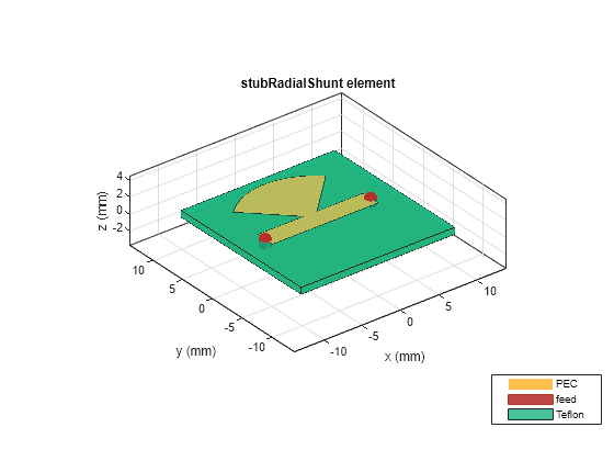
Figure contains an axes object. The axes object with title stubRadialShunt element, xlabel x (mm), ylabel y (mm) contains 8 objects of type patch, surface. These objects represent PEC, feed, Teflon.

Plot the charge distribution at 5 GHz.

charge(stub, 5e9)
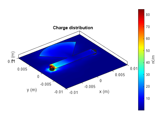
Figure contains an axes object. The axes object with title Charge distribution, xlabel x (m), ylabel y (m) contains 6 objects of type patch.

Plot the current distribution at 5 GHz.

figure
current(stub, 5e9)
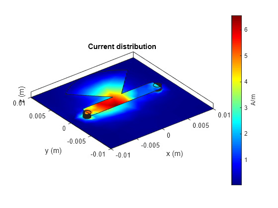
Figure contains an axes object. The axes object with title Current distribution, xlabel x (m), ylabel y (m) contains 6 objects of type patch.

Calculate and plot the s-parameters.

spar = sparameters(stub,linspace(3e9,5e9,30));
rfplot(spar)
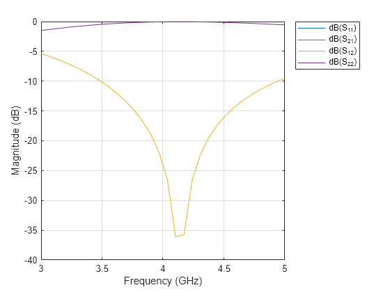
Figure contains an axes object. The axes object with xlabel Frequency (GHz), ylabel Magnitude (dB) contains 4 objects of type line. These objects represent dB(S_{11}), dB(S_{21}), dB(S_{12}), dB(S_{22}).