Fit PK Parameters Using SimBiology Problem-Based Workflow
This example shows how to estimate PK parameters of a SimBiology® model using a problem-based approach.
Load a synthetic data set. It contains drug plasma concentration data measured in both central and peripheral compartments.
load('data10_32R.mat')Convert the data set to a groupedData object.
gData = groupedData(data);
gData.Properties.VariableUnits = ["","hour","milligram/liter","milligram/liter"];
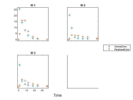
Display the data.
sbiotrellis(gData,"ID","Time",["CentralConc","PeripheralConc"],...
            Marker="+",LineStyle="none");
Use the built-in PK library to construct a two-compartment model with infusion dosing and first-order elimination. Use the configset object to turn on unit conversion.
pkmd                 = PKModelDesign;
pkc1                 = addCompartment(pkmd,"Central");
pkc1.DosingType      = "Infusion";
pkc1.EliminationType = "linear-clearance";
pkc1.HasResponseVariable = true;
pkc2                 = addCompartment(pkmd,"Peripheral");
model2cpt            = construct(pkmd);
configset            = getconfigset(model2cpt);
configset.CompileOptions.UnitConversion = true;
Assume every individual receives an infusion dose at time = 0, with a total infusion amount of 100 mg at a rate of 50 mg/hour. For details on setting up different dosing strategies, see Doses in SimBiology Models.
dose             = sbiodose("dose","TargetName","Drug_Central");
dose.StartTime   = 0;
dose.Amount      = 100;
dose.Rate        = 50;
dose.AmountUnits = "milligram";
dose.TimeUnits   = "hour";
dose.RateUnits   = "milligram/hour";
Create a problem object.
problem = fitproblem
problem =
  fitproblem with properties:

   Required:
                   Data: [0×0 groupedData]
              Estimated: [1×0 estimatedInfo]
            FitFunction: "sbiofit"
                  Model: [0×0 SimBiology.Model]
            ResponseMap: [1×0 string]

   Optional:
                  Doses: [0×0 SimBiology.Dose]
           FunctionName: "auto"
                Options: []
           ProgressPlot: 0
            UseParallel: 0
               Variants: [0×0 SimBiology.Variant]
             ErrorModel: "constant"

   sbiofit options:
                 Pooled: "auto"
    SensitivityAnalysis: "auto"
                Weights: []
Define the required properties of the object.
problem.Data        = gData;
problem.Estimated   = estimatedInfo(["log(Central)","log(Peripheral)","Q12","Cl_Central"],InitialValue=[1 1 1 1]);
problem.Model       = model2cpt;
problem.ResponseMap = ["Drug_Central = CentralConc","Drug_Peripheral = PeripheralConc"];
Define the dose to be applied during fitting.
problem.Doses = dose;
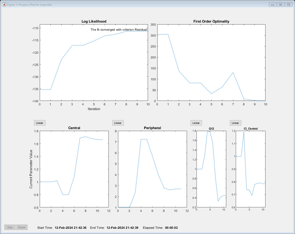
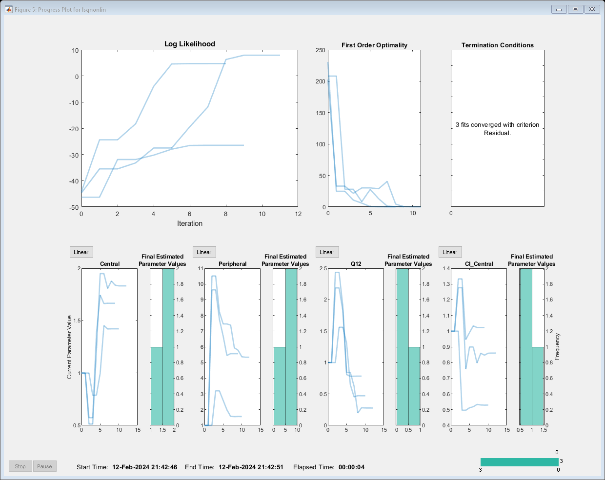
Show the progress of the estimation.
problem.ProgressPlot = true;
Fit the model to all of the data pooled together: that is, estimate one set of parameters for all individuals by setting the Pooled property to true.
problem.Pooled = true;
Perform the estimation using the fit function of the object.
pooledFit = fit(problem);
Display the estimated parameter values.
pooledFit.ParameterEstimates
ans=4×3 table
         Name         Estimate    StandardError
    ______________    ________    _____________

    {'Central'   }     1.6627        0.16569
    {'Peripheral'}     2.6864         1.0644
    {'Q12'       }    0.44945        0.19943
    {'Cl_Central'}    0.78497       0.095621
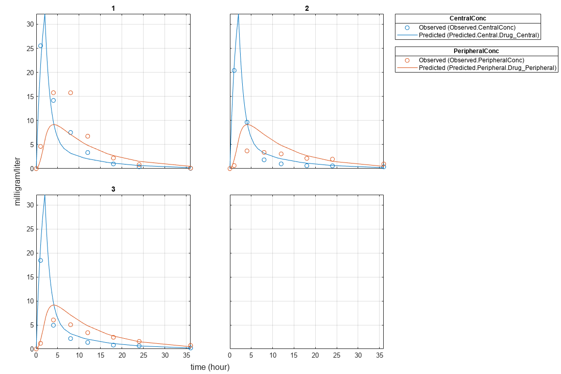
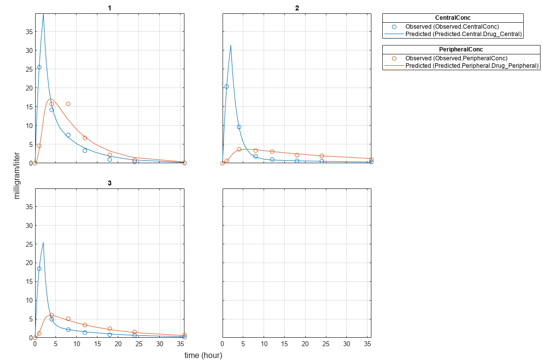
Plot the fitted results.
plot(pooledFit);
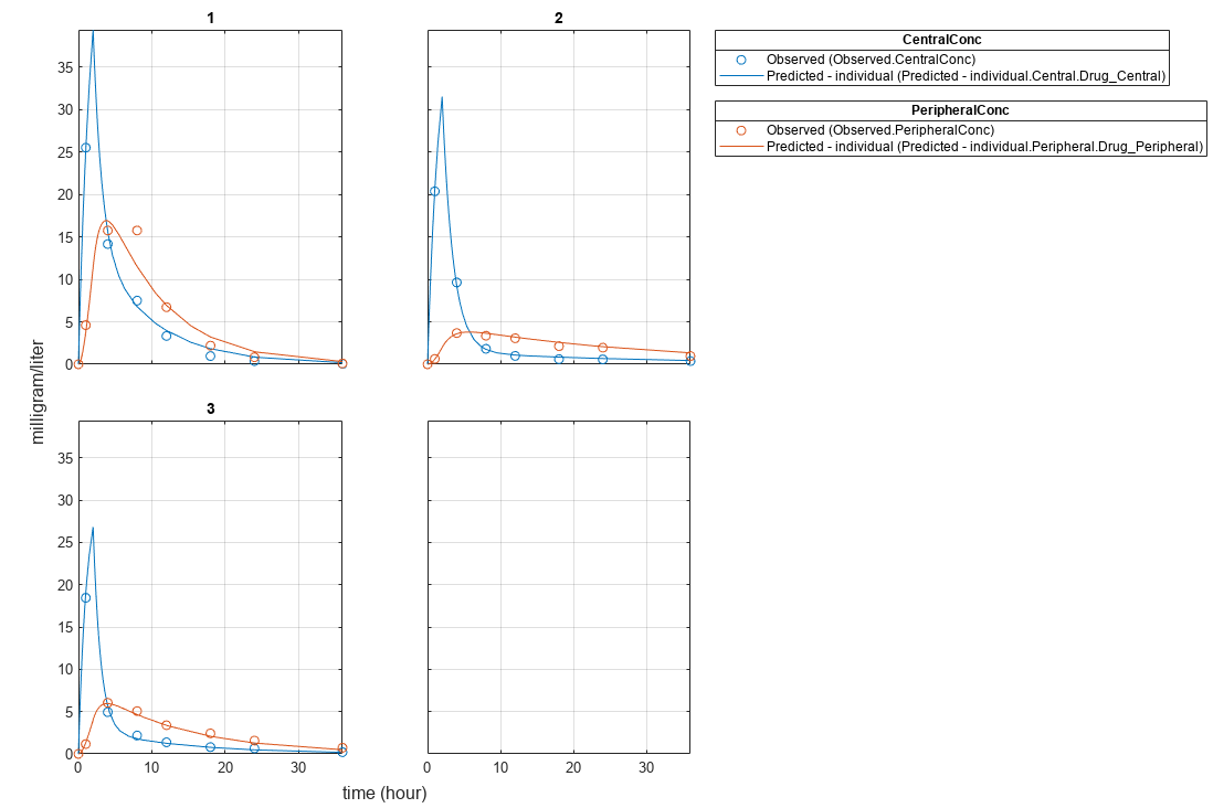
Estimate one set of parameters for each individual and see if the parameter estimates improve.
problem.Pooled  = false;
unpooledFit     = fit(problem);
Display the estimated parameter values.
unpooledFit.ParameterEstimates
ans=4×3 table
         Name         Estimate    StandardError
    ______________    ________    _____________

    {'Central'   }      1.422        0.12334
    {'Peripheral'}     1.5619        0.36355
    {'Q12'       }    0.47163        0.15196
    {'Cl_Central'}     0.5291       0.036978
ans=4×3 table
         Name         Estimate    StandardError
    ______________    ________    _____________

    {'Central'   }     1.8322       0.019672
    {'Peripheral'}     5.3364        0.65327
    {'Q12'       }     0.2764       0.030799
    {'Cl_Central'}    0.86035       0.026257
ans=4×3 table
         Name         Estimate    StandardError
    ______________    ________    _____________

    {'Central'   }     1.6657       0.038529
    {'Peripheral'}     5.5632        0.37063
    {'Q12'       }    0.78361       0.058657
    {'Cl_Central'}     1.0233       0.027311
plot(unpooledFit);
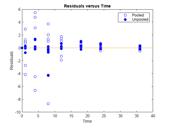
Generate a plot of the residuals over time to compare the pooled and unpooled fit results. The figure indicates unpooled fit residuals are smaller than those of the pooled fit, as expected. In addition to comparing residuals, other rigorous criteria can be used to compare the fitted results.
t = [gData.Time;gData.Time];
res_pooled = vertcat(pooledFit.R);
res_pooled = res_pooled(:);
res_unpooled = vertcat(unpooledFit.R);
res_unpooled = res_unpooled(:);
figure;
plot(t,res_pooled,"o",MarkerFaceColor="w",markerEdgeColor="b")
hold on
plot(t,res_unpooled,"o",MarkerFaceColor="b",markerEdgeColor="b")
refl = refline(0,0); % A reference line representing a zero residual
title("Residuals versus Time");
xlabel("Time");
ylabel("Residuals");
legend(["Pooled","Unpooled"]);
As illustrated, the unpooled fit accounts for variations due to the specific subjects in the study, and, in this case, the model fits better to the data. However, the pooled fit returns population-wide parameters. As an alternative, if you want to estimate population-wide parameters while considering individual variations, you can perform nonlinear mixed-effects (NLME) estimation by setting problem.FitFunction to sbiofitmixed.
problem.FitFunction = "sbiofitmixed";NLMEResults = fit(problem);
Display the estimated parameter values.
NLMEResults.IndividualParameterEstimates
ans=12×3 table
    Group         Name         Estimate
    _____    ______________    ________

      1      {'Central'   }     1.4623
      1      {'Peripheral'}     1.5306
      1      {'Q12'       }     0.4587
      1      {'Cl_Central'}    0.53208
      2      {'Central'   }      1.783
      2      {'Peripheral'}     6.6623
      2      {'Q12'       }     0.3589
      2      {'Cl_Central'}     0.8039
      3      {'Central'   }     1.7135
      3      {'Peripheral'}     4.2844
      3      {'Q12'       }    0.54895
      3      {'Cl_Central'}     1.0708
Plot the fitted results.
plot(NLMEResults);
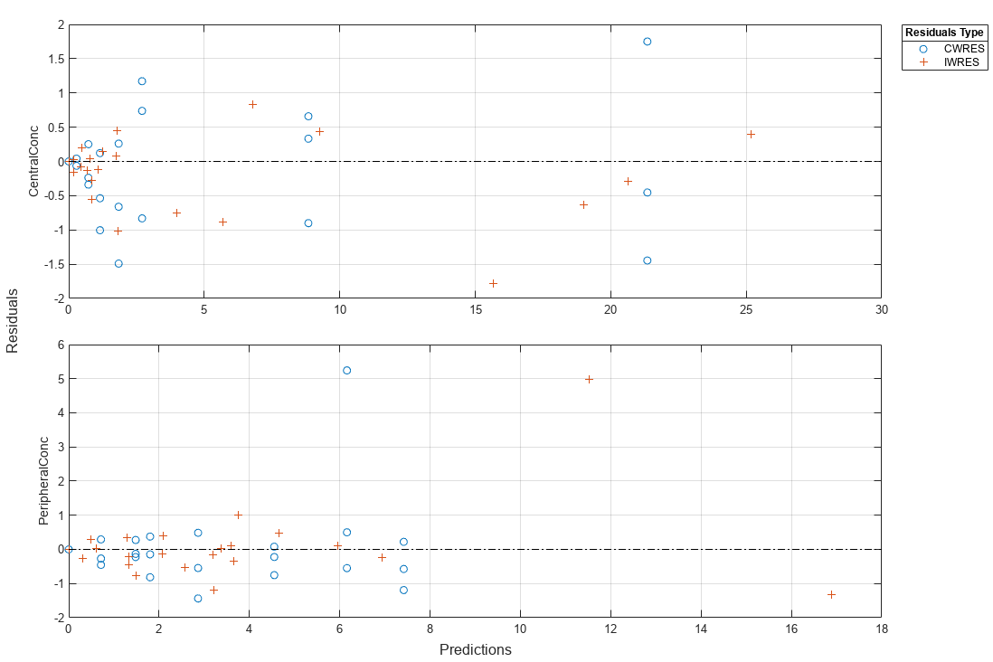
Plot the conditional weighted residuals (CWRES) and individual weighted residuals (IWRES) of model predicted values.
plotResiduals(NLMEResults,'predictions')