Enforce Safety Constraints with Control Barrier Functions

A barrier certificate defines a safety set of the desired states of a system. A control barrier function is used to find a safe control such that the states remain in the safety set. Many real-world systems operate under physical or safety constraints such as state boundaries. Control barrier functions (CBFs) enforce safety constraints by keeping system states inside a defined safe set while a baseline controller tracks performance goals.

Using Simulink^® Control Design™ software, you can enforce CBF safety constraints by restricting control inputs in real time. For safety constraints expressed as a linear inequality in u, the software solves a quadratic program (QP) at each step to apply the closest control that satisfies safety and actuator bounds. Therefore, CBFs provide formal safety guarantees and integrate easily with your existing baseline control system. You can use CBFs for applications where safety-critical operation is essential and constraints must always be respected, such as autonomous driving and robotic safety.

Control Barrier Functions

Consider control-affine plant dynamics of the following form.

$$\dot{x}=f(x)+g(x)u$$

The control barrier function h(x) defines a safety set $$\{x:h(x)\ge 0\}$$, that is, an invariant set where any trajectory starting inside the set remains within the set.

For h(x) , the Lie derivative is the time derivative along the system trajectories, defined as follows.

$$\dot{h}(x)=\frac{\partial h(x)}{\partial x}\dot{x}=\underset{L_{f}h(x)}{\underbrace{\frac{\partial h(x)}{\partial x}f(x)}}+\underset{L_{g}h(x)}{\underbrace{\frac{\partial h(x)}{\partial x}g(x)}}u$$

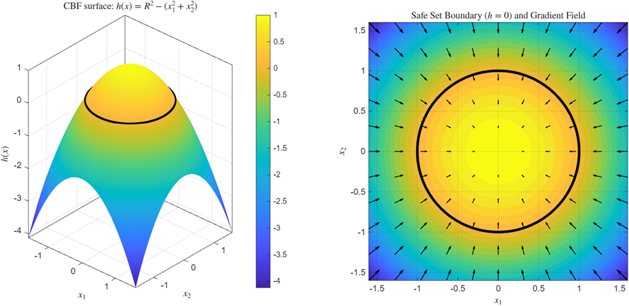
For example, this figure shows a simple barrier function surface and its safe set. The barrier function h(x) defines a circular safe region where h(x) ≥ 0. The 3D plot shows the surface of h(x), while the 2D contour plot highlights the safe set boundary h = 0, and the gradient field, which points toward increasing h. This figure illustrates how CBFs maintain forward invariance by keeping the system state within the region where the barrier function is nonnegative.

Relative Degree and Higher-Order Lie Derivatives

Relative degree is the number of time derivatives of h you must take before the control term u appears explicitly. This means, for a relative degree of 1:

$$\begin{array}{l}\dot{h}(x)=L_{f}h(x)+L_{g}h(x)u\\ L_{g}h(x)\ne 0\end{array}$$

When the control term does not appear in the first-order Lie derivative of the CBF (L_gh = 0), you can use higher-order derivatives of the CBF. That is, you must differentiate further along f(x) until the input term u appears in the r-th order time derivative.

$$h^r(x)=L_f^{r}h(x)+L_g{L}_f^{r-1}h(x)u$$

The function h(x) has a higher relative degree r until the following condition is satisfied.

$$L_g{L}_f^{r-1}h(x)\ne 0$$

Additionally, you obtain the higher-order Lie derivatives by repeatedly differentiating along the fields f(x) and g(x). Use these derivatives to build constraints for a higher relative degree.

• L_fⁱh is the i-th Lie derivative of h_x with respect to x, with $$L_{f}h(x)=\frac{\partial h}{\partial x}f(x)$$ and $$L_f^{i}h(x)=\frac{\partial L_f^{i-1}h(x)}{\partial x}f(x)$$.

• L_gL_fⁱh is given by $$L_g{L}_f^{i}h(x)=\frac{\partial L_f^{i}h(x)}{\partial x}g(x)$$.

Control Barrier Function Constraints

The control barrier function constraint for relative degree 1 is described by:

$$\dot{h}(x,u)\ge -\alpha (h(x))$$

Here α(h(x)) is an extended class Κ function. Typically, this function is of the following form.

$$\alpha (h(x))=\gamma h^{\beta }(x)$$

Therefore, in standard form, you can write the CBF inequality as:

$$L_{f}h(x)+L_{g}h(x)u\ge -\gamma h^{\beta }$$

Here, γ is the constraint factor and β is the constraint power.

High-Order Control Barrier Functions

If L_gh = 0, then you must use a higher-order formulation of the CBF constraints, described as follows:

$$h^r(x,u)\ge -\alpha (h(x))$$

For high-order CBF, you can use the exponential high-order CBF formulation that enforces a strict state-dependent high-relative degree safety for nonlinear systems. h(x) is an exponential CBF if there exists a row vector K_α such that:

$$L_f^{r}h(x)+L_g{L}_f^{r-1}h(x)u\ge -K_{\alpha }{\eta }_h$$

Here:

$${\eta }_h=\left[\begin{array}{c}h(x)\\ L_{f}h(x)\\ ⋮\\ L_f^{r-1}h(x)\end{array}\right].$$

You obtain this row vector of gains K_α using pole placement to make the companion form Hurwitz stable. This ensures all derivatives of h(x) decay exponentially.

An exponential CBF constraint is defined as follows:

$$L_f^{r}h(x)+L_g{L}_f^{r-1}h(x)u\ge -{\displaystyle \sum _{i=0}^{r-1}{\gamma }_i{L}_f^{i}h(x)}$$

Here, γ_i is the constraint factor values computed by placing poles for desired decay rate. The software also allows you to specify a more general form of high-order CBF constraints defined as follows:

$$L_f^{r}h(x)+L_g{L}_f^{r-1}h(x)u\ge -{\displaystyle \sum _{i=0}^{r-1}{\gamma }_{i+1}{(L_f^{i}h)}^{{\beta }_{i+1}}(x)}$$

For this form, you explicitly specify the values for constraint factors γ_i and the constraint power β.

Using CBF Constraints in Simulink

Use these blocks to implement control barrier function constraints in Simulink.

• Barrier Certificate Enforcement block — For relative degree 1.

• High-Order Control Barrier Function block — For relative degree 1 to 4.

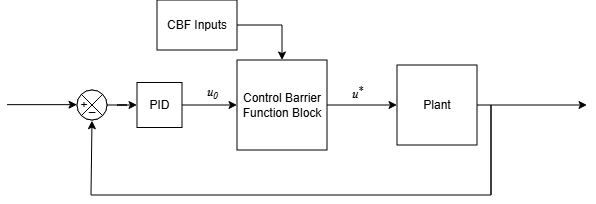
These blocks, which require Optimization Toolbox™ software, compute minimum deviation control from baseline controller subject to barrier certificate constraints and action bounds. The blocks use a quadratic programming (QP) solver to find the control action u that minimizes the function $${\left|u-u_0\right|}^2$$ in real time. Here, u₀ is the unmodified control action from the controller.

This table summarizes the constraints used by the blocks, based on relative degree.

Barrier Function Relative Degree	Constraint Equation
First order	$$\begin{array}{l}{L}_{f}h+L_{g}hu+{\gamma }_1{h}^{{\beta }_1}\ge 0\\ u_{\min }\le u\le u_{\max }\end{array}$$
Second order	$$\begin{array}{l}{L}_f^{2}h+L_g{L}_{f}hu+{\gamma }_1{h}^{{\beta }_1}+{\gamma }_2{(}^{L_f}\ge 0\\ u_{\min }\le u\le u_{\max }\end{array}$$
Third order	$$\begin{array}{l}{L}_f^{3}h+L_g{L}_f^{2}hu+{\gamma }_1{h}^{{\beta }_1}+{\gamma }_2{(}^{L_f}+{\gamma }_3{(}^{L_f^2}\ge 0\\ u_{\min }\le u\le u_{\max }\end{array}$$
Fourth order	$$\begin{array}{l}{L}_f^{4}h+L_g{L}_f^{3}hu+{\gamma }_1{h}^{{\beta }_1}+{\gamma }_2{(}^{L_f}+{\gamma }_3{(}^{L_f^2}+{\gamma }_4{(}^{L_f^3}\ge 0\\ u_{\min }\le u\le u_{\max }\end{array}$$

Implementation Workflow

To implement CBF constraints, use these steps.

1. Define the system dynamics in control-affine form $$\dot{x}=f(x)+g(x)u$$.

2. Define a control barrier function h(x) that encodes the desired safety constraint.

3. Determine the relative degree by differentiating h(x) until the input term u appears explicitly.

4. Compute the required Lie derivatives and provide them as block inputs.

5. Connect the baseline controller input u₀ and the optional action bounds u_min and u_max.

6. Tune the parameters.

   • For standard CBF, configure the constraint factor γ and constraint power β to modify the aggressiveness of the constraint.

   • For exponential CBF, set the pole values for the exponential decay rate.

This figure shows how to add the CBF block to your existing system with baseline controller. The block inputs depend on the relative degree of the constraint.

Since the blocks modify the original control action, the final closed-loop system might not achieve the design objectives of the original controller, such as stability margins.

You must verify that the combined controller and CBF blocks meet your original control objectives. If the system does not meet your original objectives, consider updating your original controller design. For example, you can add additional gain and phase margins to compensate for any potential performance degradation.

Examples

• Enforce Barrier Certificate Constraints for PID Controllers — Implements a simple first-order CBF.

• Enforce Barrier Certificate Constraints for Collision-Free Multi-Robot System — Defines a barrier function such that the robots reach their target position while maintaining a distance greater than a threshold distance between any two robots.

• Safe PID Controller for Two Link Robot using High-Order Control Barrier Function — Computes higher‑order derivatives and uses exponential CBF.

References

[1] Xiao, Wei, and Calin Belta. “High-Order Control Barrier Functions.” IEEE Transactions on Automatic Control 67, no. 7 (2022): 3655–62. https://doi.org/10.1109/TAC.2021.3105491.