Design Optimization Using Lookup Table Requirements for Gain Scheduling (Code)
This example shows how to tune parameters in a lookup table in a model that uses gain scheduling to adjust the controller response to a plant that varies. Model tuning uses the sdo.optimize command.
Ship Steering Model
Open the Simulink® Model.
mdl = 'sdoShipSteering';
open_system(mdl)
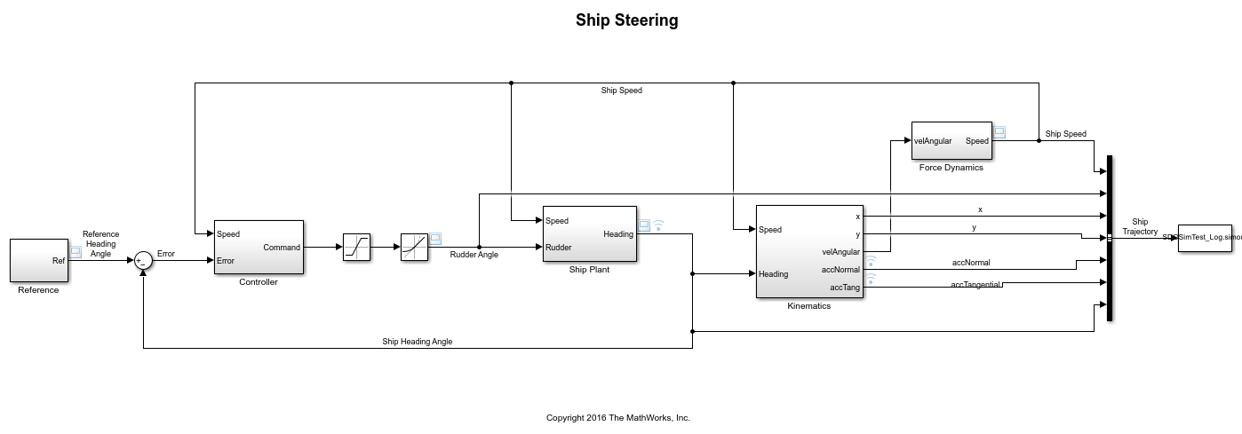
This model implements the Nomoto model which is commonly used for ship steering. The dynamic characteristics of a ship vary significantly with factors such as the ship speed. Therefore the rudder controller should also vary with speed, in order to meet requirements for steering the ship.
To keep the ship on course, a control loop compares the ship's heading angle with the reference heading angle, and a PD controller sends command signals to the rudder. The Ship Plant block implements the Nomoto model, a second order system whose parameters vary with the ship's speed. The ship is initially traveling at its maximum speed of 15 m/s, but it will slow down when the reference trajectory specifies a turn in the water. This turning, along with the force of the engine, is used by the Force Dynamics block to compute the speed of the ship over time. The Kinematics block computes the trajectory of the ship.
Open the Controller block.
open_system([mdl '/Controller'])
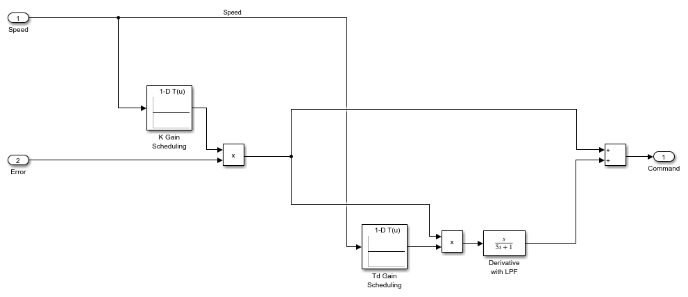
When the speed changes, the ship plant also changes. Therefore the PD controller gains need to change, and speed is used as the scheduling variable. The controller is in the form K(1 + sTd) where K is the overall gain and Td is the time constant associated with the derivative term. Gain scheduling is implemented via lookup tables, and the table data are specified by K and Td. These are vectors which specify different values for different speeds. The different speeds are specified in the lookup table breakpoint vectors bpK and bpTd.
Design Problem
The reference specifies that at 200 seconds, the ship should turn 180 degrees and reverse course. One requirement is that the ship heading angle needs to match the reference heading angle within an envelope. For the safety and comfort of passengers, a second requirement is that the total acceleration of the ship needs to stay within a bound of 0.25 g, where 1 g is the acceleration of gravity at Earth's surface, 9.8 m/s/s.
The controller parameter vectors K and Td will be design variables, and will be tuned to try to meet the requirements. If it is not possible to meet both requirements, then the lookup table breakpoints bpK and bpTd will also be used as design variables. In that case, we will need to specify an additional requirement that bpK and bpTd must be monotonically strictly increasing, because this is required for breakpoint vectors in Simulink lookup tables.
Specify Design Requirements
Specify the requirements which must be satisfied. First, the ship should follow the reference trajectory. Since the reference is essentially a step change from 0 to 180 degrees, you specify a step response envelope for the ship heading angle.
Requirements = struct;
Requirements.StepResponseEnvelope = sdo.requirements.StepResponseEnvelope(...
    'StepTime',200, ...  (seconds)
    'RiseTime',75, ...
    'SettlingTime',200, ...
    'PercentRise',85, ...  (%)
    'PercentOvershoot',5, ...
    'PercentSettling',1, ...
    'FinalValue',pi ...   (radians)
    );
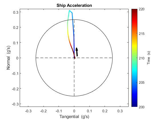
The second requirement is that for the safety and comfort of passengers, the total acceleration should not exceed 0.25 g's at any time. The total acceleration is composed of two components, a tangential component along the direction of the ship's motion, and a normal (horizontal) component. The requirement that total acceleration not exceed 0.25 g's corresponds to requiring that in the phase plane of tangential and normal acceleration, this ship's trajectory remain within a circle of radius 0.25*9.8.
accelGravity = 9.8;
Requirements.Comfort = sdo.requirements.PhasePlaneEllipse(...
     'Radius', 0.25*[1 1] * accelGravity);
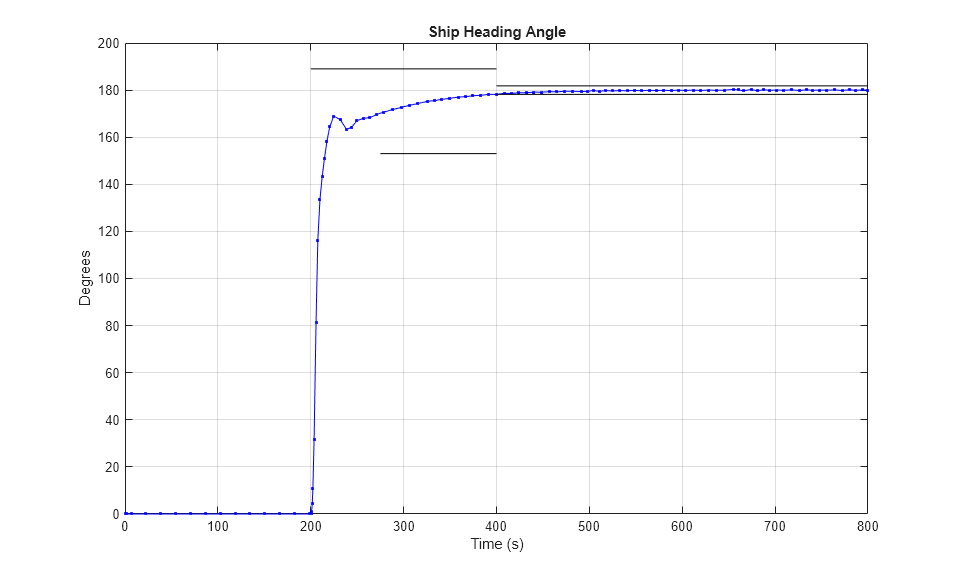
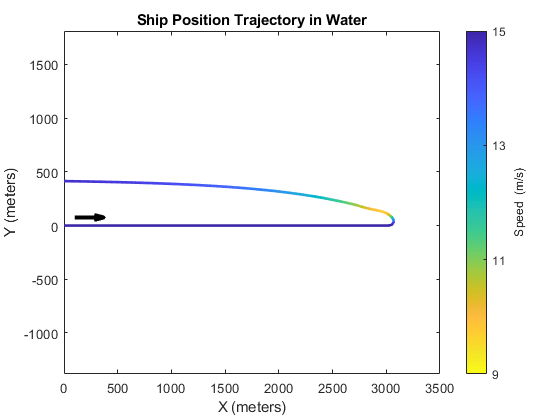
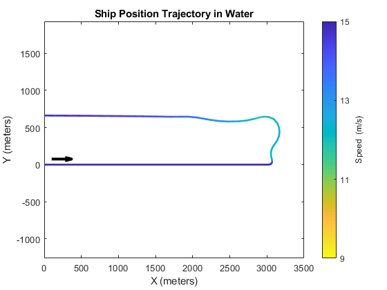
Examine the behavior of the ship with the initial, untuned controller parameters, to see whether the requirements are satisfied. Use the function sdoShipSteeringPlots to plot the ship's behavior. The first plot below shows that the ship's heading angle stays within the tolerance bounds of the step response envelope, satisfying the first requirement. The second plot shows the trajectory of the ship in the water. The black arrow indicates the starting position and direction of motion. The ship turns 180 degrees and the diameter is approximately 415 meters. The third plot shows the ship acceleration in the phase plane of tangential and normal acceleration. The black arrow indicates the starting point and direction of evolution over time. The total acceleration exceeds the bound near 208 seconds, so the requirement for passenger safety and comfort is not satisfied.
hPlots = sdoShipSteeringPlots(mdl,Requirements);
Specify Design Variables
Specify the design variables to be tuned by the optimization routine in order to satisfy the requirements. Specify the gains of the PD controller, K and Td, as design variables. For initial values, use -0.1 for all entries in the K vector, and 50 for all entries in the Td vector. If the requirements can't all be satisfied, then later the breakpoint vectors bpK and bpTd can also be design variables.
DesignVars = sdo.getParameterFromModel(mdl,{'K','Td'});
DesignVars(1).Value = -0.1*[1 1 1 1];
DesignVars(2).Value =  50*[1 1 1 1];
sdo.setValueInModel(mdl,DesignVars);
Create Optimization Objective Function
Create an objective function that will be called at each optimization iteration to evaluate the design requirements as the design variables are tuned. This cost function has input arguments for the model, design variables, simulator (defined below), and design requirements. The cost function uses the maximum of the Comfort requirements at all times when it is computed, in order to consolidate requirement evaluation results to a scalar so the number of elements is the same regardless of time steps taken by the Simulink solver.
type sdoShipSteering_Design
function Vals = sdoShipSteering_Design(mdl, P, Simulator, Requirements)
%SDOSHIPSTEERING_DESIGN Objective function for ship steering
%
% Function called at each iteration of the optimization problem.
%
% The function is called with the model named mdl, a set of parameter
% values, P, a Simulator, and the design Requirements to evaluate.  It
% returns the objective value and constraint violations, Vals, to the
% optimization solver.
%
% See the sdoExampleCostFunction function and sdo.optimize for a more
% detailed description of the function signature.
%
% See also sdoShipSteering_cmddemo

% Copyright 2016 The MathWorks, Inc.

%% Model Evaluation

% Simulate the model.
Simulator.Parameters = P;
Simulator = sim(Simulator);

% Retrieve logged signal data.
SimLog = find(Simulator.LoggedData,get_param(mdl, 'SignalLoggingName'));
Heading     = find(SimLog, 'Heading');
NormalAccel = find(SimLog, 'NormalAccel');
TangenAccel = find(SimLog, 'TangenAccel');

% Evaluate the step response envelope requirement
Cleq_StepResponseEnvelope = evalRequirement(Requirements.StepResponseEnvelope, Heading.Values);

% Evaluate the safety/comfort requirement on total acceleration.
Cleq_Comfort = evalRequirement(Requirements.Comfort, NormalAccel.Values, TangenAccel.Values);

%% Return Values.

% Collect the evaluated design requirement values in a structure to return
% to the optimization solver.
Vals.Cleq = Cleq_StepResponseEnvelope(:);
Vals.Cleq = [Vals.Cleq  ; Cleq_Comfort];

% Evaluate monotonic variable requirement
if isfield(Requirements, 'Monotonic')
    Cleq_bpK  = evalRequirement(Requirements.Monotonic, P(3).Value);
    Cleq_bpTd = evalRequirement(Requirements.Monotonic, P(4).Value);
    Vals.Cleq = [Vals.Cleq ; Cleq_bpK ; Cleq_bpTd];
end

end
The cost function requires a Simulator to run the model. Create the simulator and add model signals to log, so their values are available to the cost function.
Simulator = sdo.SimulationTest(mdl);

% Ship Heading Angle
Heading = Simulink.SimulationData.SignalLoggingInfo;
Heading.BlockPath = 'sdoShipSteering/Ship Plant';
Heading.LoggingInfo.LoggingName = 'Heading';
Heading.LoggingInfo.NameMode = 1;
Heading.OutputPortIndex = 1;

% Normal Acceleration
NormalAccel = Simulink.SimulationData.SignalLoggingInfo;
NormalAccel.BlockPath = 'sdoShipSteering/Kinematics';
NormalAccel.LoggingInfo.LoggingName = 'NormalAccel';
NormalAccel.LoggingInfo.NameMode = 1;
NormalAccel.OutputPortIndex = 4;

% Tangential Acceleration
TangenAccel = Simulink.SimulationData.SignalLoggingInfo;
TangenAccel.BlockPath = 'sdoShipSteering/Kinematics';
TangenAccel.LoggingInfo.LoggingName = 'TangenAccel';
TangenAccel.LoggingInfo.NameMode = 1;
TangenAccel.OutputPortIndex = 5;

% Collect logged signals
Simulator.LoggingInfo.Signals = [...
    Heading ; ...
    NormalAccel ; ...
    TangenAccel ];
Optimize Lookup Table Data
Before optimizing, configure the simulator for optimization and enable fast restart.
Simulator = setup(Simulator,FastRestart='on');
During optimization, the Simulink solver can generate a warning if the size of the time step becomes too small. Temporarily suppress this warning.
warnState = warning('query','Simulink:Engine:SolverMinStepSizeWarn');
warnState1 = warning('query','Simulink:Solver:Warning');
warnState2 = warning('query','SimulinkExecution:DE:MinStepSizeWarning');
warning('off','Simulink:Engine:SolverMinStepSizeWarn');
warning('off','Simulink:Solver:Warning');
warning('off','SimulinkExecution:DE:MinStepSizeWarning');
To optimize, define a handle to the cost function that uses the Simulator and Requirements defined above. Use an anonymous function that takes one argument (the design variables) and calls the objective function. Finally, call sdo.optimize to optimize the design variables to try to meet the requirements.
optimfcn = @(P) sdoShipSteering_Design(mdl,P,Simulator,Requirements);
[Optimized_DesignVars,Info] = sdo.optimize(optimfcn,DesignVars);
 Optimization started 2026-Apr-19, 06:50:03

                               max                     First-order
 Iter F-count        f(x)   constraint    Step-size    optimality
    0     17            0       0.6127
    1     34            0       0.3215        0.865        0.321
    2     57            0       0.3079        0.174        0.308
    3    103            0       0.3079      0.00127        0.308
Converged to an infeasible point.

fmincon stopped because the size of the current step is less than
the value of the step size tolerance but constraints are not
satisfied to within the value of the constraint tolerance.
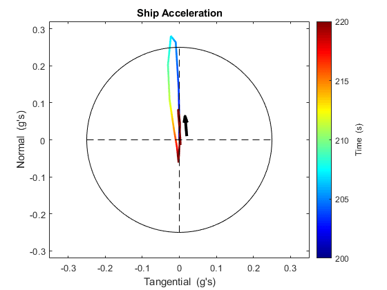
The display indicates that the optimizer was not able to satisfy all requirements. Try the optimized design variables in the model and plot the results. The heading angle is not within the required step response envelope, and the total acceleration still exceeds the allowable level during part of the turn. In addition, the turning diameter has increased to 660 meters, so the turn is not as tight as with untuned gains.
sdo.setValueInModel(mdl,Optimized_DesignVars);
hPlots = sdoShipSteeringPlots(mdl,Requirements,hPlots);

Optimize Lookup Table Data and Breakpoints
To try to meet the design requirements, use the optimization result from above as the start point, and tune additional variables. Add breakpoints bpK and bpTd as design variables. The ship's maximum speed is 15 m/s, and during turning it may slow to 60% of the maximum speed, or 9 m/s. Set the breakpoint initial values to be equally spaced between 9 and 15 m/s. Constrain the breakpoint minimum values to 9 m/s, and constrain the breakpoint maximum values to 15 m/s.
DesignVars = Optimized_DesignVars;
DesignVars(3:4) = sdo.getParameterFromModel(mdl,{'bpK','bpTd'});

% Set initial values
DesignVars(3).Value = [9 11 13 15];
DesignVars(4).Value = [9 11 13 15];

% Constrain min and max values
DesignVars(3).Minimum = 9;
DesignVars(3).Maximum = 15;
DesignVars(4).Minimum = 9;
DesignVars(4).Maximum = 15;

% Set values in the model
sdo.setValueInModel(mdl,DesignVars);
Breakpoints in the Simulink lookup table block must be strictly monotonically increasing. Add this to the design requirements.
Requirements.Monotonic = sdo.requirements.MonotonicVariable;
optimfcn = @(P) sdoShipSteering_Design(mdl, P, Simulator, Requirements);
Optimize the model by tuning all four design variables, to see if all requirements can be met.
[Optimized_DesignVars, Info] = sdo.optimize(optimfcn,DesignVars);
 Optimization started 2026-Apr-19, 06:50:27

                               max                     First-order
 Iter F-count        f(x)   constraint    Step-size    optimality
    0     29            0       0.3079
    1     63            0       0.1432        0.148         1.01
    2     98            0      0.03626       0.0858        0.597
    3    128            0      0.01911       0.0548       0.0859
    4    159            0     0.007837       0.0341      0.00627
    5    190            0            0       0.0256     0.000903
Local minimum found that satisfies the constraints.

Optimization completed because the objective function is non-decreasing in
feasible directions, to within the value of the optimality tolerance,
and constraints are satisfied to within the value of the constraint tolerance.
The display indicates that the optimizer was able to satisfy all requirements. Restore the simulator and model settings modified by the setup function, which includes disabling fast restart.
Simulator = restore(Simulator);
Try the optimized design variables in the model and plot the results. In the plots below, the heading angle is within the step response envelope, and the total acceleration is within the allowed range of 0.25 g's. In addition, the turning diameter is 615 meters, which is tighter than when breakpoints were not tuned.
sdo.setValueInModel(mdl,Optimized_DesignVars);
hPlots = sdoShipSteeringPlots(mdl,Requirements,hPlots);


In this example, the ship plant varied with the ship speed, so the controller gains also needed to vary. Gain scheduling was implemented using lookup tables. By tuning the gains and breakpoint values in the controller, the ship was able to follow the reference heading angle, while also constraining total acceleration to ensure a safe and comfortable ride for passengers.
Related Examples
To learn how to optimize the lookup tables in the gain scheduled controller using the Response Optimizer, see Design Optimization Using Lookup Table Requirements for Gain Scheduling (GUI).
Restore the state of warnings.
warning(warnState);
warning(warnState1);
warning(warnState2);
See Also
sdo.requirements.FunctionMatching | sdo.requirements.MonotonicVariable | sdo.requirements.PhasePlaneEllipse | sdo.requirements.PhasePlaneRegion | sdo.requirements.RelationalConstraint | sdo.requirements.SmoothnessConstraint