Assemble a Gear Model
The examples that follow show how to position and orient gear bodies so that they satisfy the assembly requirements of the various gear constraint blocks. Each example starts with an overview of relevant gear dimensions and frame placements. These attributes guide the selection of rigid transforms needed to ensure that the gears assemble in mesh.
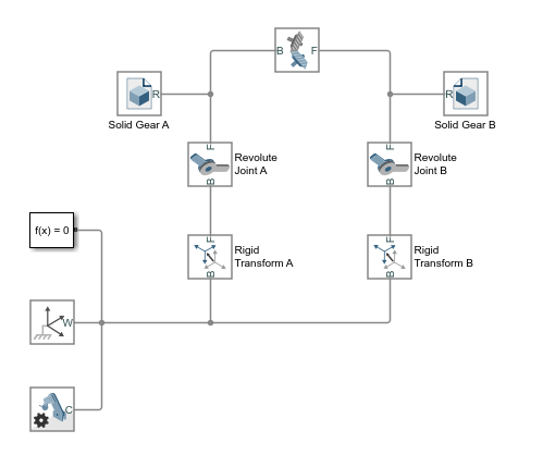
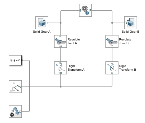
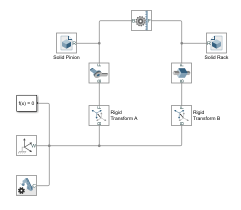
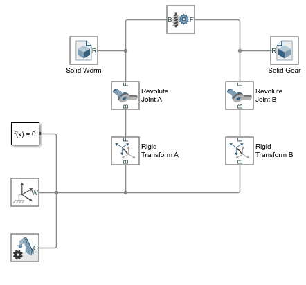
The models share the same block diagram topology, with the model components—bodies, joints, and gear constraint—arranged in a kinematic loop in each case. The figure shows a simple loop. The carrier body is in the examples considered to be fixed to the world frame, with its inertia consequently reduced to a superfluous detail and the body altogether ignored.
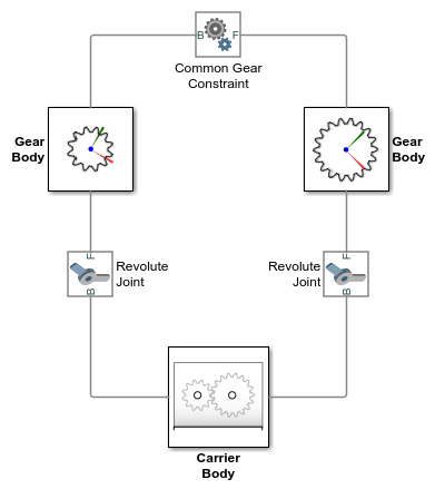
The models comprise four types of Simscape™ Multibody™ blocks:
File Solid — Provides the gear geometries, inertias, and colors. The gear geometries, complete with teeth or threads to more clearly show the gears in mesh, are imported from STEP files. The poses of the gear reference frames relative to the gear geometries are obtained from the same files.
Joint — Provides the gear bodies with the requisite degrees of freedom. Revolute Joint blocks enable rotation about a single axis. Prismatic Joint blocks enable translation along a single axis. Velocity state targets specified in the joint blocks set the gears in motion.
Rigid Transform — Rotates and translates the joints and the attached gear bodies so that they are properly placed for meshing. Rigid Transform blocks provide the means to change the gear placements and therefore to satisfy the gear assembly requirements.
Gear constraint — Couples the motions of the gear bodies. Gear constraint blocks eliminate one degree of freedom between the gears, causing them to move as though in mesh. The examples showcase, one by one, the various gear constraint blocks.
Bevel Gear

The DocBevelGearStart model provides an example of a bevel gear assembly. To open the model, at the MATLAB® command prompt, enter:
openExample('sm/DocGearModelExample','supportingFile','DocBevelGearStart.slx')
The model, based on the Bevel Gear Constraint block, is complete in every sense but one—all rigid transforms are zero and the gear reference frames are therefore coincident in space.
This short tutorial shows how suitable transforms follow readily from the gear dimensions and assembly constraints—and how, once specified in the Rigid Transform blocks, they enable the gear model to assemble as though in mesh without error.
Gear Geometry
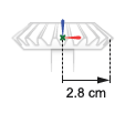
The bevel gears, A and B, are identical in size, with a pitch radius of 2.8 cm in each case. The gear reference frames are placed with origins at the gear centers and z-axes aligned with the gear rotation axes so as to face away from the gear shafts. This alignment is consistent with the Revolute Joint blocks, which allow rotation about the z-axis only.
Gear Assembly
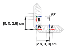
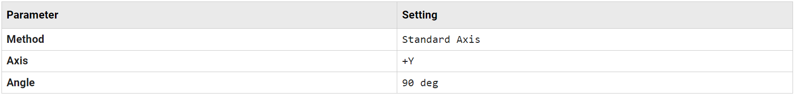
The gear rotation axes meet at a right angle. The reference frame of bevel gear A sits at an offset of [2.8, 0, 0] cm, in Cartesian coordinates, relative to the world frame. The reference frame of bevel gear B sits at an offset of [0, 0, 2.8] cm relative to the world frame and at an angle of 90 deg about the y-axis also of the world frame.
Complete the Model
Complete the bevel gear model by specifying the rigid transforms described in the gear assembly schematic. The conceptual animation that follows shows the incremental effects that the rigid transforms would have were they to apply in sequence during model update.
If you have not yet done so, open the incomplete bevel gear model by entering:
openExample('sm/DocGearModelExample','supportingFile','DocBevelGearStart.slx')
In the Rigid Transform A block dialog box, specify the Translation parameters shown in the table. These parameters set the position of bevel gear A relative to the world frame as described in the Gear Assembly schematic.

In the Rigid Transform B block dialog box, specify the Translation parameters shown in the table. These parameters set the position of bevel gear B relative to the world frame as described in the Gear Assembly schematic.

In the Rigid Transform B block dialog box, specify the Rotation parameters shown in the table. These parameters set the orientation of bevel gear B relative to the world frame as described in the Gear Assembly schematic.
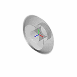
Simulate the model. Multibody Explorer opens with the dynamic gear visualization shown at the beginning of this example. To see a complete bevel gear model, at the MATLAB command prompt enter:
openExample('sm/DocGearModelExample','supportingFile','DocBevelGear.slx')
Simscape Multibody opens a bevel gear model with the rigid transforms described in this example.
External Spur Gear
The DocCommonGearExternalStart model provides an example of an external spur gear assembly. To open the model, at the MATLAB command prompt, enter:
openExample('sm/DocGearModelExample','supportingFile','DocCommonGearExternalStart.slx')
The model, based on the Common Gear Constraint block, is complete in every sense but one—all rigid transforms are zero and the gear reference frames are therefore coincident in space.
This short tutorial shows how suitable transforms follow readily from the gear dimensions and assembly constraints—and how, once specified in the Rigid Transform blocks, they enable the gear model to assemble as though in mesh without error.
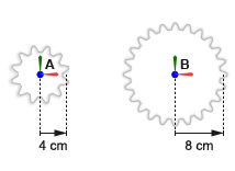
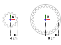
Gear Geometry
The small spur gear, A, has a pitch radius of 4 cm. The large spur gear, B, has a pitch radius of 8 cm. The gear reference frames are placed with origins at the gear centers and z-axes aligned with the gear rotation axes so as to face away from the gear shafts. This alignment is consistent with the Revolute Joint block, which allows rotation about the z-axis only.
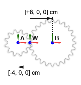
Gear Assembly
The spur gear rotation axes are parallel to each other. The reference frame of the small spur gear sits at an offset of [-4, 0, 0] cm, in Cartesian coordinates, relative to the world frame. The reference frame of the large spur gear sits at an offset of [-8, 0, 0] cm, also relative to the world frame.
Complete the Model
Complete the external spur gear model by specifying the rigid transforms described in the gear assembly schematic. The conceptual animation that follows shows the incremental effects that the rigid transforms would have were they to apply in sequence during model update.
If you have not yet done so, open the incomplete external spur gear model by entering:
openExample('sm/DocGearModelExample','supportingFile','DocCommonGearExternalStart.slx')
In the Rigid Transform A block dialog box, specify the Translation parameters shown in the table. These parameters set the position of the small spur gear, A, relative to the world frame as described in the Gear Assembly schematic.

In the Rigid Transform B block dialog box, specify the Translation parameters shown in the table. These parameters set the position of the large spur gear, B, relative to the world frame as described in the Gear Assembly schematic.

Simulate the model. Multibody Explorer opens with the dynamic gear visualization shown at the beginning of this example. To see a complete external spur gear model, at the MATLAB command prompt enter:
openExample('sm/DocGearModelExample','supportingFile','DocCommonGearExternal.slx')
Internal Spur Gear
The DocCommonGearInternalStart model provides an example of an internal spur gear assembly. To open the model, at the MATLAB command prompt, enter:
openExample('sm/DocGearModelExample','supportingFile','DocCommonGearInternalStart.slx')
The model, based on the Common Gear Constraint block, is complete in every sense but one—all rigid transforms are zero and the gear reference frames are therefore coincident in space.

This short tutorial shows how suitable transforms follow readily from the gear dimensions and assembly constraints—and how, once specified in the Rigid Transform blocks, they enable the gear model to assemble as though in mesh without error.
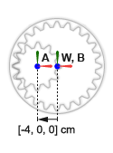
Gear Geometry
The spur gear, A, has a pitch radius of 4 cm. The ring gear, B, has a pitch radius of 8 cm. The gear reference frames are placed with origins at the gear centers and z-axes aligned with the gear rotation axes so as to face away from the gear shafts. This alignment is consistent with the Revolute Joint block, which allows rotation about the z-axis only.
Gear Assembly
The gear rotation axes are parallel to each other. The spur gear reference frame sits at an offset of [-4, 0, 0] cm, in Cartesian notation, relative to the world frame. The ring gear reference frame sits left with its origin and z-axis coincident with those of the world frame.
Complete the Model
Complete the internal spur gear model by specifying the rigid transforms described in the gear assembly schematic. The conceptual animation that follows shows the incremental effects that the rigid transforms would have were they to apply in sequence during model update.

If you have not yet done so, open the incomplete internal spur gear model by entering:
openExample('sm/DocGearModelExample','supportingFile','DocCommonGearInternalStart.slx')
In the Rigid Transform A block dialog box, specify the Translation parameters shown in the table. These parameters set the position of the spur gear, A, relative to the world frame as described in the Gear Assembly schematic.

Simulate the model. Multibody Explorer opens with the dynamic gear visualization shown at the beginning of this example. To see a complete internal spur gear model, at the MATLAB command prompt, enter:
openExample('sm/DocGearModelExample','supportingFile','DocCommonGearInternal.slx')
Rack and Pinion
The DocRackAndPinionStart model provides an example of a rack-and-pinion assembly. To open the model, at the MATLAB command prompt, enter:
openExample('sm/DocGearModelExample','supportingFile','DocRackAndPinionStart.slx')
The model, based on the Rack and Pinion Constraint block, is complete in every sense but one—all rigid transforms are zero and the gear reference frames are therefore coincident in space.
This short tutorial shows how suitable transforms follow readily from the gear dimensions and assembly constraints—and how, once specified in the Rigid Transform blocks, they enable the gear model to assemble as though in mesh without error.
Gear Geometry
The pinion, A, has a pitch radius of 2 cm. The pinion reference frame is placed with origin at the pinion center and z-axis along the pinion axis. The rack reference frame is placed with origin 3.75 cm from the rack edge and z-axis along the rack length. The frame alignments are consistent with the Revolute Joint and Prismatic Joint blocks, which allow motion about or along the z-axis only.
Gear Assembly
The rack translation axis is at a right angle to the pinion rotation axis. The pinion reference frame sits at an offset of [0, 2, 0] cm, in Cartesian notation, relative to the world frame. The rack reference frame sits at an angle of 90 deg relative to the positive y-axis of the world frame.

Complete the Model
Complete the rack-and-pinion model by specifying the rigid transforms described in the gear assembly schematic. The conceptual animation that follows shows the incremental effects that the rigid transforms would have were they to apply in sequence during model update.
If you have not yet done so, open the incomplete rack-and-pinion model by entering:
openExample('sm/DocGearModelExample','supportingFile','DocRackAndPinionStart.slx')
In the Rigid Transform A block dialog box, specify the Translation parameters shown in the table. These parameters set the position of the pinion, A, relative to the world frame as described in the Gear Assembly schematic.

In the Rigid Transform B block dialog box, specify the Rotation parameters shown in the table. These parameters set the orientation of the rack, B, relative to the world frame as described in the Gear Assembly schematic.
Simulate the model. Multibody Explorer opens with the dynamic gear visualization shown at the beginning of this example. To see a complete rack-and-pinion model, at the MATLAB command prompt enter:
openExample('sm/DocGearModelExample','supportingFile','DocRackAndPinion.slx')
Worm and Gear
The DocWormAndGearStart model provides an example of a worm-and-gear assembly. To open the model, at the MATLAB command prompt, enter:
openExample('sm/DocGearModelExample','supportingFile','DocWormAndGearStart.slx')
The model, based on the Worm and Gear Constraint block, is complete in every sense but one—all rigid transforms are zero and the gear reference frames are therefore coincident in space.
This short tutorial shows how suitable transforms follow readily from the gear dimensions and assembly constraints—and how, once specified in the Rigid Transform blocks, they enable the gear model to assemble as though in mesh without error.
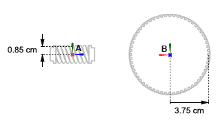
Gear Geometry
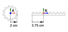
The worm, A, has a pitch radius of 0.85 cm. The gear, B, has a pitch radius of 3.75 cm. The worm and gear reference frames are placed with origins at the geometry centers and z-axes aligned with the respective rotation axes. This alignment is consistent with the Revolute Joint block, which allows rotation about the z-axis only.
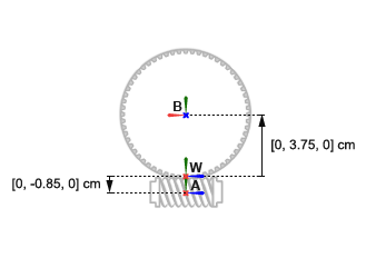
Gear Assembly
The worm rotation axis is at a right angle to the gear rotation axis. The worm reference frame sits at an offset of [0, -0.85, 0] cm, in Cartesian notation, relative to the world frame. The gear reference frame sits at an offset of [0, +3.75, 0] cm and at an angle of 90 deg about the positive y-axis relative to the world frame.
Complete the Model
Complete the worm-and-gear model by specifying the rigid transforms described in the gear assembly schematic. The conceptual animation that follows shows the incremental effects that the rigid transforms would have were they to apply in sequence during model update.
If you have not yet done so, open the incomplete worm-and-gear model by entering:
openExample('sm/DocGearModelExample','supportingFile','DocWormAndGearStart.slx')
In the Rigid Transform A block dialog box, specify the Translation parameters shown in the table. These parameters set the position of the worm, A, relative to the world frame as described in the Gear Assembly schematic.

In the Rigid Transform A block dialog box, specify the Translation parameters shown in the table. These parameters set the position of the gear, B, relative to the world frame as described in the Gear Assembly schematic.

In the Rigid Transform B block dialog box, specify the Rotation parameters shown in the table. These parameters set the orientation of the gear, B, relative to the world frame as described in the Gear Assembly schematic.

Simulate the model. Multibody Explorer opens with the dynamic gear visualization shown at the beginning of this example. To see a complete worm-and-gear gear model, at the MATLAB command prompt, enter:
openExample('sm/DocGearModelExample','supportingFile','DocWormAndGear.slx')