Implement Incremental Learning for Regression Using Succinct Workflow

This example shows how to use the succinct workflow to implement incremental learning for linear regression with prequential evaluation. Specifically, this example does the following:

1. Create a default incremental learning model for linear regression.

2. Simulate a data stream using a for loop, which feeds small chunks of observations to the incremental learning algorithm.

3. For each chunk, use updateMetricsAndFit to measure the model performance given the incoming data, and then fit the model to that data.

Create Default Model Object

Create a default incremental learning model for linear regression.

Mdl = incrementalRegressionLinear()

Mdl = 
  incrementalRegressionLinear

               IsWarm: 0
              Metrics: [1x2 table]
    ResponseTransform: 'none'
                 Beta: [0x1 double]
                 Bias: 0
              Learner: 'svm'

Mdl.EstimationPeriod

ans = 
1000

Mdl is an incrementalRegressionLinear model object. All its properties are read-only.

Mdl must be fit to data before you can use it to perform any other operations. The software sets the estimation period to 1000 because half the width of the epsilon insensitive band Epsilon is unknown. You can set Epsilon to a positive floating-point scalar by using the 'Epsilon' name-value pair argument. This action results in a default estimation period of 0.

Load Data

Load the robot arm data set.

load robotarm

For details on the data set, enter Description at the command line.

Implement Incremental Learning

Use the succinct workflow to update model performance metrics and fit the incremental model to the training data by calling the updateMetricsAndFit function. At each iteration:

• Process 50 observations to simulate a data stream.

• Overwrite the previous incremental model with a new one fitted to the incoming observations.

• Store the cumulative metrics, window metrics, and the first coefficient ${\beta }_1$ to see how they evolve during incremental learning.

% Preallocation
n = numel(ytrain);
numObsPerChunk = 50;
nchunk = floor(n/numObsPerChunk);
ei = array2table(zeros(nchunk,2),'VariableNames',["Cumulative" "Window"]);
beta1 = zeros(nchunk,1);    

% Incremental fitting
for j = 1:nchunk
    ibegin = min(n,numObsPerChunk*(j-1) + 1);
    iend   = min(n,numObsPerChunk*j);
    idx = ibegin:iend;    
    Mdl = updateMetricsAndFit(Mdl,Xtrain(idx,:),ytrain(idx));
    ei{j,:} = Mdl.Metrics{"EpsilonInsensitiveLoss",:};
    beta1(j + 1) = Mdl.Beta(1);
end

IncrementalMdl is an incrementalRegressionLinear model object trained on all the data in the stream. During incremental learning and after the model is warmed up, updateMetricsAndFit checks the performance of the model on the incoming observations, and then fits the model to those observations.

Inspect Model Evolution

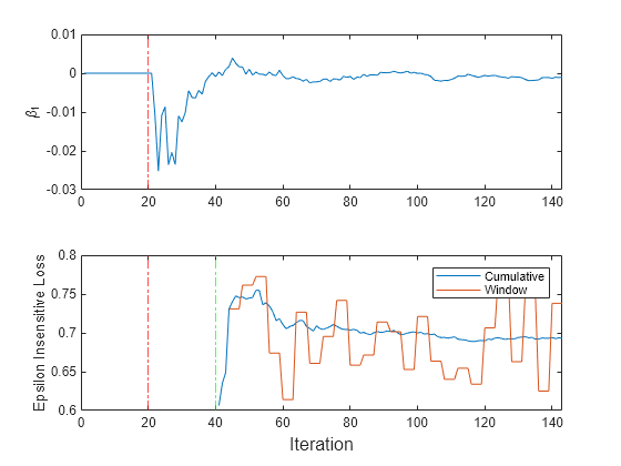
To see how the performance metrics and ${\beta }_1$ evolve during training, plot them on separate tiles.

t = tiledlayout(2,1);
nexttile
plot(beta1)
ylabel('\beta_1')
xlim([0 nchunk])
xline(Mdl.EstimationPeriod/numObsPerChunk,'r-.')
nexttile
h = plot(ei.Variables);
xlim([0 nchunk])
ylabel('Epsilon Insensitive Loss')
xline(Mdl.EstimationPeriod/numObsPerChunk,'r-.')
xline((Mdl.EstimationPeriod + Mdl.MetricsWarmupPeriod)/numObsPerChunk,'g-.')
legend(h,ei.Properties.VariableNames)
xlabel(t,'Iteration')

The plot suggests that updateMetricsAndFit does the following:

• After the estimation period (first 20 iterations), fit ${\beta }_1$ during all incremental learning iterations.

• Compute the performance metrics after the metrics warm-up period only.

• Compute the cumulative metrics during each iteration.

• Compute the window metrics after processing 200 observations (4 iterations).