Initialize Incremental Learning Model from SVM Regression Model Trained in Regression Learner
This example shows how to tune and train a linear SVM regression model using the Regression Learner app. Then, at the command line, initialize and train an incremental model for linear SVM regression using the information gained from training in the app.
Load and Preprocess Data
Load the 2015 NYC housing data set, and shuffle the data. For more details on the data, see NYC Open Data.
load NYCHousing2015
rng(1); % For reproducibility
n = size(NYCHousing2015,1);
idxshuff = randsample(n,n);
NYCHousing2015 = NYCHousing2015(idxshuff,:);
For numerical stability, scale SALEPRICE by 1e6.
NYCHousing2015.SALEPRICE = NYCHousing2015.SALEPRICE/1e6;
Consider training a linear SVM regression model to about 1% of the data, and reserving the remaining data for incremental learning.
Regression Learner supports categorical variables. However, models for
incremental learning require dummy-coded categorical variables. Because the
BUILDINGCLASSCATEGORY and NEIGHBORHOOD variables
contain many levels (some with low representation), the probability that a partition does
not have all categories is high. Therefore, dummy-code all categorical variables.
Concatenate the matrix of dummy variables to the rest of the numeric variables.
catvars = ["BOROUGH" "BUILDINGCLASSCATEGORY" "NEIGHBORHOOD"];
dumvars = splitvars(varfun(@(x)dummyvar(categorical(x)),NYCHousing2015, ...
      'InputVariables',catvars));
NYCHousing2015(:,catvars) = [];
idxnum = varfun(@isnumeric,NYCHousing2015,'OutputFormat','uniform');
NYCHousing2015 = [dumvars NYCHousing2015(:,idxnum)];
Randomly partition the data into 1% and 99% subsets by calling cvpartition and specifying a holdout (test) sample proportion of 0.99. Create tables for the 1% and 99% partitions.
cvp = cvpartition(n,'HoldOut',0.99);
idxtt = cvp.training;
idxil = cvp.test;
NYCHousing2015tt = NYCHousing2015(idxtt,:);
NYCHousing2015il = NYCHousing2015(idxil,:);
Tune and Train Model Using Regression Learner
Open Regression Learner by entering regressionLearner at the command line.
regressionLearner
Alternatively, on the Apps tab, click the Show more arrow to open the apps gallery. Under Machine Learning and Deep Learning, click the app icon.
Choose the training data set and variables.
On the Regression Learner tab, in the File section, select New Session, and then select From Workspace.
In the New Session from Workspace dialog box, under Data Set Variable, select the data set NYCHousing2015tt.
Under Response, ensure the response variable SALEPRICE is selected.
Click Start Session.
The app implements 5-fold cross-validation by default.
Train a linear SVM regression model. Tune only the Epsilon hyperparameter by using Bayesian optimization.
On the Regression Learner tab, in the Models section, click the Show more arrow to open the apps gallery. In the Support Vector Machines section, click Optimizable SVM.
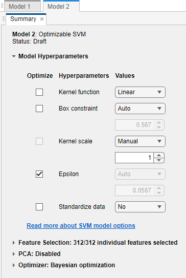
On the model Summary tab, in the Model Hyperparameters section:
Deselect the Optimize boxes for all available options except Epsilon.
Set the value of Kernel scale to
Manualand1.Set the value of Standardize data to
No.

On the Regression Learner tab, in the Train section, click Train All and select Train Selected.
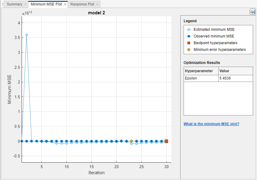
The app shows a plot of the generalization minimum MSE of the model as optimization progresses. The app can take some time to optimize the algorithm.

Export the trained, optimized linear SVM regression model.
On the Regression Learner tab, in the Export section, select Export Model, and select Export Model.
In the Export Model dialog box, click OK.
The app passes the trained model, among other variables, in the structure array trainedModel to the workspace. Close Regression Learner .
Convert Exported Model to Incremental Model
At the command line, extract the trained SVM regression model from trainedModel.
Mdl = trainedModel.RegressionSVM;
Convert the model to an incremental model.
IncrementalMdl = incrementalLearner(Mdl)
IncrementalMdl.Epsilon
IncrementalMdl =

  incrementalRegressionLinear

               IsWarm: 1
              Metrics: [1×2 table]
    ResponseTransform: 'none'
                 Beta: [312×1 double]
                 Bias: 12.3802
              Learner: 'svm'


  Properties, Methods


ans =

    5.4536
IncrementalMdl is an incrementalRegressionLinear model object for incremental learning using a linear SVM regression model. incrementalLearner initializes IncrementalMdl using the coefficients and the optimized value of the Epsilon hyperparameter learned from Mdl. Therefore, you can predict responses by passing IncrementalMdl and data to predict. Also, the IsWarm property is true, which means that the incremental learning functions measure the model performance from the start of incremental learning.
Implement Incremental Learning
Because incremental learning functions accept floating-point matrices only, create matrices for the predictor and response data.
Xil = NYCHousing2015il{:,1:(end-1)};
Yil = NYCHousing2015il{:,end};
Perform incremental learning on the 99% data partition by using the updateMetricsAndFit function. Simulate a data stream by processing 500 observations at a time. At each iteration:
Call
updateMetricsAndFitto update the cumulative and window epsilon insensitive loss of the model given the incoming chunk of observations. Overwrite the previous incremental model to update the losses in theMetricsproperty.Store the losses and last estimated coefficient β313.
% Preallocation
nil = sum(idxil);
numObsPerChunk = 500;
nchunk = floor(nil/numObsPerChunk);
ei = array2table(zeros(nchunk,2),'VariableNames',["Cumulative" "Window"]);
beta313 = [IncrementalMdl.Beta(end); zeros(nchunk,1)];

% Incremental learning
for j = 1:nchunk
    ibegin = min(nil,numObsPerChunk*(j-1) + 1);
    iend   = min(nil,numObsPerChunk*j);
    idx = ibegin:iend;
    IncrementalMdl = updateMetricsAndFit(IncrementalMdl,Xil(idx,:),Yil(idx));
    ei{j,:} = IncrementalMdl.Metrics{"EpsilonInsensitiveLoss",:};
    beta313(j + 1) = IncrementalMdl.Beta(end);
end
IncrementalMdl is an incrementalRegressionLinear model object trained on all the data in the stream.
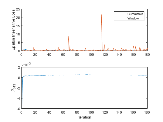
Plot a trace plot of the performance metrics and estimated coefficient β313.
figure
subplot(2,1,1)
h = plot(ei.Variables);
xlim([0 nchunk])
ylabel('Epsilon Insensitive Loss')
legend(h,ei.Properties.VariableNames)
subplot(2,1,2)
plot(beta313)
ylabel('\beta_{313}')
xlim([0 nchunk])
xlabel('Iteration')

The cumulative loss gradually changes with each iteration (chunk of 500 observations), whereas the window loss jumps. Because the metrics window is 200 by default, updateMetricsAndFit measures the performance based on the latest 200 observations in each 500 observation chunk.
β313 changes abruptly and then levels off as updateMetricsAndFit processes chunks of observations.