eqn =
Main Content
Results for
I have a problem with the movement of a pawn by two fields in its first move does anyone have a suggestion for a solution
function chess_game()
% Funkcja główna inicjalizująca grę w szachy
% Inicjalizacja stanu gry
gameState = struct();
gameState.board = initialize_board();
gameState.currentPlayer = 'white';
gameState.selectedPiece = [];
% Utworzenie GUI
fig = figure('Name', 'Gra w Szachy', 'NumberTitle', 'off', 'MenuBar', 'none', 'UserData', gameState);
ax = axes('Parent', fig, 'Position', [0 0 1 1], 'XTick', [], 'YTick', []);
axis(ax, [0 8 0 8]);
hold on;
% Wyświetlenie planszy
draw_board(ax, gameState.board);
% Obsługa kliknięcia myszy
set(fig, 'WindowButtonDownFcn', @(src, event)on_click(ax, src));
end
function board = initialize_board()
% Inicjalizuje planszę z ustawieniem początkowym figur
board = {
'R', 'N', 'B', 'Q', 'K', 'B', 'N', 'R';
'P', 'P', 'P', 'P', 'P', 'P', 'P', 'P';
'', '', '', '', '', '', '', '';
'', '', '', '', '', '', '', '';
'', '', '', '', '', '', '', '';
'', '', '', '', '', '', '', '';
'p', 'p', 'p', 'p', 'p', 'p', 'p', 'p';
'r', 'n', 'b', 'q', 'k', 'b', 'n', 'r';
};
end
function draw_board(~, board)
% Rysuje szachownicę i figury
colors = [1 1 1; 0.8 0.8 0.8];
for row = 1:8
for col = 1:8
% Rysowanie pól
rectColor = colors(mod(row + col, 2) + 1, :);
rectangle('Position', [col-1, 8-row, 1, 1], 'FaceColor', rectColor, 'EdgeColor', 'k');
% Rysowanie figur
piece = board{row, col};
if ~isempty(piece)
text(col-0.5, 8-row+0.5, piece, 'HorizontalAlignment', 'center', ...
'FontSize', 20, 'FontWeight', 'bold');
end
end
end
end
function on_click(ax, fig)
% Funkcja obsługująca kliknięcia myszy
pos = get(ax, 'CurrentPoint');
x = floor(pos(1,1)) + 1; % Zaokrąglij współrzędne w poziomie i dopasuj do indeksów
y = 8 - floor(pos(1,2)); % Dopasuj współrzędne w pionie (odwrócenie osi Y)
% Pobranie stanu gry z figury
gameState = get(fig, 'UserData');
if x >= 1 && x <= 8 && y >= 1 && y <= 8
disp(['Kliknięto na pole: (', num2str(x), ', ', num2str(y), ')']);
if isempty(gameState.selectedPiece)
% Wybór figury
piece = gameState.board{y, x};
if ~isempty(piece)
if (strcmp(gameState.currentPlayer, 'white') && any(ismember(piece, 'RNBQKP'))) || ...
(strcmp(gameState.currentPlayer, 'black') && any(ismember(piece, 'rnbqkp')))
gameState.selectedPiece = [y, x];
disp(['Wybrano figurę: ', piece, ' na pozycji (', num2str(x), ', ', num2str(y), ')']);
else
disp('Nie możesz wybrać tej figury.');
end
else
disp('Nie wybrano figury.');
end
else
% Sprawdzenie, czy kliknięto ponownie na wybraną figurę
if isequal(gameState.selectedPiece, [y, x])
disp('Anulowano wybór figury.');
gameState.selectedPiece = [];
else
% Ruch figury
[sy, sx] = deal(gameState.selectedPiece(1), gameState.selectedPiece(2));
piece = gameState.board{sy, sx};
if is_valid_move(gameState.board, piece, [sy, sx], [y, x], gameState.currentPlayer)
% Wykonanie ruchu
gameState.board{sy, sx} = ''; % Usuwamy figurę z poprzedniego pola
gameState.board{y, x} = piece; % Umieszczamy figurę na nowym polu
gameState.selectedPiece = [];
% Przełącz gracza
gameState.currentPlayer = switch_player(gameState.currentPlayer);
% Odśwież planszę
cla(ax);
draw_board(ax, gameState.board);
else
disp('Ruch niezgodny z zasadami.');
end
end
end
% Zaktualizowanie stanu gry w figurze
set(fig, 'UserData', gameState);
end
end
function valid = is_valid_move(board, piece, from, to, currentPlayer)
% Funkcja sprawdzająca, czy ruch jest poprawny
[sy, sx] = deal(from(1), from(2));
[dy, dx] = deal(to(1), to(2));
dy_diff = dy - sy;
dx_diff = abs(dx - sx);
targetPiece = board{dy, dx};
% Sprawdzenie, czy ruch jest w granicach planszy
if dx < 1 || dx > 8 || dy < 1 || dy > 8
valid = false;
return;
end
% Nie można zbijać swoich figur
if ~isempty(targetPiece) && ...
((strcmp(currentPlayer, 'white') && ismember(targetPiece, 'RNBQKP')) || ...
(strcmp(currentPlayer, 'black') && ismember(targetPiece, 'rnbqkp')))
valid = false;
return;
end
% Zasady ruchu dla każdej figury
switch lower(piece)
case 'p' % Pion
direction = strcmp(currentPlayer, 'white') * 2 - 1; % 1 dla białych, -1 dla czarnych
startRow = strcmp(currentPlayer, 'white') * 2 + 1; % Rząd startowy dla białych i czarnych
if isempty(targetPiece)
% Ruch o jedno pole do przodu
if dy_diff == direction && dx_diff == 0
valid = true;
% Ruch o dwa pola do przodu z pozycji startowej
elseif dy_diff == 2 * direction && dx_diff == 0 && sy == startRow
if isempty(board{sy + direction, sx}) && isempty(board{dy, dx})
valid = true;
else
valid = false;
end
else
valid = false;
end
else
% Zbijanie na ukos
valid = (dx_diff == 1) && (dy_diff == direction);
end
case 'r' % Wieża
valid = (dx_diff == 0 || dy_diff == 0) && path_is_clear(board, from, to);
case 'n' % Skoczek
valid = (dx_diff == 2 && abs(dy_diff) == 1) || (dx_diff == 1 && abs(dy_diff) == 2);
case 'b' % Goniec
valid = (dx_diff == abs(dy_diff)) && path_is_clear(board, from, to);
case 'q' % Hetman
valid = ((dx_diff == 0 || dy_diff == 0) || (dx_diff == abs(dy_diff))) && path_is_clear(board, from, to);
case 'k' % Król
valid = max(abs(dx_diff), abs(dy_diff)) == 1;
otherwise
valid = false;
end
end
function clear = path_is_clear(board, from, to)
% Sprawdza, czy ścieżka między polami jest wolna od innych figur
[sy, sx] = deal(from(1), from(2));
[dy, dx] = deal(to(1), to(2));
stepY = sign(dy - sy);
stepX = sign(dx - sx);
y = sy + stepY;
x = sx + stepX;
while y ~= dy || x ~= dx
if ~isempty(board{y, x})
clear = false;
return;
end
y = y + stepY;
x = x + stepX;
end
clear = true;
end
function nextPlayer = switch_player(currentPlayer)
% Przełącza aktywnego gracza
if strcmp(currentPlayer, 'white')
nextPlayer = 'black';
else
nextPlayer = 'white';
end
end
Speaking as someone with 31+ years of experience developing and using imshow, I want to advocate for retiring and replacing it.
The function imshow has behaviors and defaults that were appropriate for the MATLAB and computer monitors of the 1990s, but which are not the best choice for most image display situations in today's MATLAB. Also, the 31 years have not been kind to the imshow code base. It is a glitchy, hard-to-maintain monster.
My new File Exchange function, imview, illustrates the kind of changes that I think should be made. The function imview is a much better MATLAB graphics citizen and produces higher quality image display by default, and it dispenses with the whole fraught business of trying to resize the containing figure. Although this is an initial release that does not yet support all the useful options that imshow does, it does enough that I am prepared to stop using imshow in my own work.
The Image Processing Toolbox team has just introduced in R2024b a new image viewer called imageshow, but that image viewer is created in a special-purpose window. It does not satisfy the need for an image display function that works well with the axes and figure objects of the traditional MATLAB graphics system.
I have published a blog post today that describes all this in more detail. I'd be interested to hear what other people think.
Note: Yes, I know there is an Image Processing Toolbox function called imview. That one is a stub for an old toolbox capability that was removed something like 15+ years ago. The only thing the toolbox imview function does now is call error. I have just submitted a support request to MathWorks to remove this old stub.
The int function in the Symbolic Toolbox has a hold/release functionality wherein the expression can be held to delay evaluation
syms x I
eqn = I == int(x,x,'Hold',true)
which allows one to show the integral, and then use release to show the result
release(eqn)
Maybe it would be nice to be able to hold/release any symbolic expression to delay the engine from doing evaluations/simplifications that it typically does. For example:
x*(x+1)/x, sin(sym(pi)/3)
If I'm trying to show a sequence of steps to develop a result, maybe I want to explicitly keep the x/x in the first case and then say "now the x in the numerator and denominator cancel and the result is ..." followed by the release command to get the final result.
Perhaps held expressions could even be nested to show a sequence of results upon subsequent releases.
Held expressions might be subject to other limitations, like maybe they can't be fplotted.
Seems like such a capability might not be useful for problem solving, but might be useful for exposition, instruction, etc.
Watt's Up with Electric Vehicles?EV modeling Ecosystem (Eco-friendly Vehicles), V2V Communication and V2I communications thereby emitting zero Emissions to considerably reduce NOx ,Particulates matters,CO2 given that Combustion is always incomplete and will always be.
Reduction of gas emissions outside to the environment will improve human life span ,few epidemic diseases and will result in long life standard
We will be updating the MATLAB Answers infrastructure at 1PM EST today. We do not expect any disruption of service during this time. However, if you notice any issues, please be patient and try again later. Thank you for your understanding.
Hi! My name is Mike McLernon, and I’m a product marketing engineer with MathWorks. In my role, I look at the trends ongoing in the wireless industry, across lots of different standards (think 5G, WLAN, SatCom, Bluetooth, etc.), and I seek to shape and guide the software that MathWorks builds to respond to these trends. That’s all about communicating within the Mathworks organization, but every so often it’s worth communicating these trends to our audience in the world at large. Many of the people reading this are engineers (or engineers at heart), and we all want to know what’s happening in the geek world around us. I think that now is one of these times to communicate an important milestone. So, without further ado . . .
Bluetooth 6.0 is here! Announced in September by the Bluetooth Special Interest Group (SIG), it’s making more advances in its quest to create a “world without wires”. A few of the salient features in Bluetooth 6.0 are:
- Channel sounding (for accurate distance measurements)
- Decision-based advertising filtering (for more efficient channel scanning)
- Monitoring advertisers (for improved energy efficiency when devices come into and go out of range)
- Frame space updates (for both higher throughput and better coexistence management)
Bluetooth 6.0 includes other features as well, but the SIG has put special promotional emphasis on channel sounding (CS), which once upon a time was called High Accuracy Distance Measurement (HADM). The SIG has said that CS is a step towards true distance awareness, and 10 cm ranging accuracy. I think their emphasis is in exactly the right place, so let’s learn more about this technology and how it is used.
CS can be used for the following use cases:
- Keyless vehicle entry, performed by communication between a key fob or phone and the car’s anchor points
- Smart locks, to permit access only when an authorized device is within a designated proximity to the locks
- Geofencing, to limit access to designated areas
- Warehouse management, to monitor inventory and manage logistics
- Asset tracking for virtually any object of interest

In the past, Bluetooth devices would use a received signal strength indicator (RSSI) measurement to infer the distance between two of them. They would assume a free space path loss on the link, and use a straightforward equation to estimate distance:


 where
whereSo in this method,  . But if the signal suffers more loss from multipath or shadowing, then the distance would be overestimated. Something better needed to be found.
 . But if the signal suffers more loss from multipath or shadowing, then the distance would be overestimated. Something better needed to be found.
Bluetooth 6.0 introduces not one, but two ways to accurately measure distance:
- Round-trip time (RTT) measurement
- Phase-based ranging (PBR) measurement
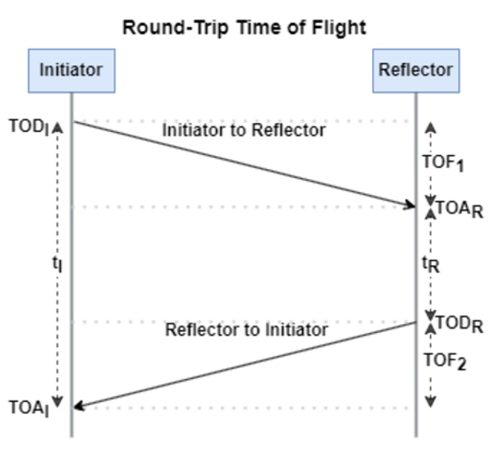
The RTT measurement method uses the fact that the Bluetooth signal time of flight (TOF) between two devices is half the RTT. It can then accurately compute the distance d as
 , where c is again the speed of light. This method requires accurate measurements of the time of departure (TOD) of the outbound signal from device 1 (the Initiator), time of arrival (TOA) of the outbound signal to device 2 (the Reflector), TOD of the return signal from device 2, and TOA of the return signal to device 1. The diagram below shows the signal paths and the times.
If you want to see how you can use MATLAB to simulate the RTT method, take a look at Estimate Distance Between Bluetooth LE Devices by Using Channel Sounding and Round-Trip Timing.
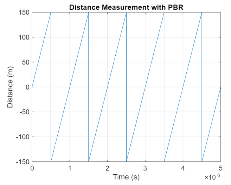
The PBR method uses two Bluetooth signals of different frequencies to measure distance. These signals are simply tones – sine waves. Without going through the derivation, PBR calculates distance d as
The mod() operation is needed to eliminate ambiguities in the distance calculation and the final division by two is to convert a round trip distance to a one-way distance. Because a given phase difference value can hold true for an infinite number of distance values, the mod() operation chooses the smallest distance that satisfies the equation. Also, these tones can be as close as 1 MHz apart. In that case, the maximum resolvable distance measurement is about 150 m. The plot below shows that ambiguity and repetition in distance measurement.
If you want to see how you can use MATLAB to simulate the PBR method, take a look at Estimate Distance Between Bluetooth LE Devices by Using Channel Sounding and Phase-Based Ranging.
Bluetooth 6.0 outlines RTT and PBR distance measurement methods, but CS does not mandate a specific algorithm for calculating distance estimates. This flexibility allows device manufacturers to tailor solutions to various use cases, balancing computational complexity with required accuracy and adapting to different radio environments. Examples include simple phase difference calculations and FFT-based methods.
Although Bluetooth 6.0 is now out, it is far from a finished version. The SIG is actively working through the ratification process for two major extensions:
- High Data Throughput, up to 8 Mbps
- 5 and 6 GHz operation
See the last few minutes of this video from the SIG to learn more about these exciting future developments. And if you want to see more Bluetooth blogs, give a review of this one! Finally, if you have specific Bluetooth questions, give me a shout and let’s start a discussion!
I am very excited to share my new book "Data-driven method for dynamic systems" available through SIAM publishing: https://epubs.siam.org/doi/10.1137/1.9781611978162
This book brings together modern computational tools to provide an accurate understanding of dynamic data. The techniques build on pencil-and-paper mathematical techniques that go back decades and sometimes even centuries. The result is an introduction to state-of-the-art methods that complement, rather than replace, traditional analysis of time-dependent systems. One can find methods in this book that are not found in other books, as well as methods developed exclusively for the book itself. I also provide an example-driven exploration that is (hopefully) appealing to graduate students and researchers who are new to the subject.
Each and every example for the book can be reproduced using the code at this repo: https://github.com/jbramburger/DataDrivenDynSyst
Hope you like it!
Christmas season is underway at my house:
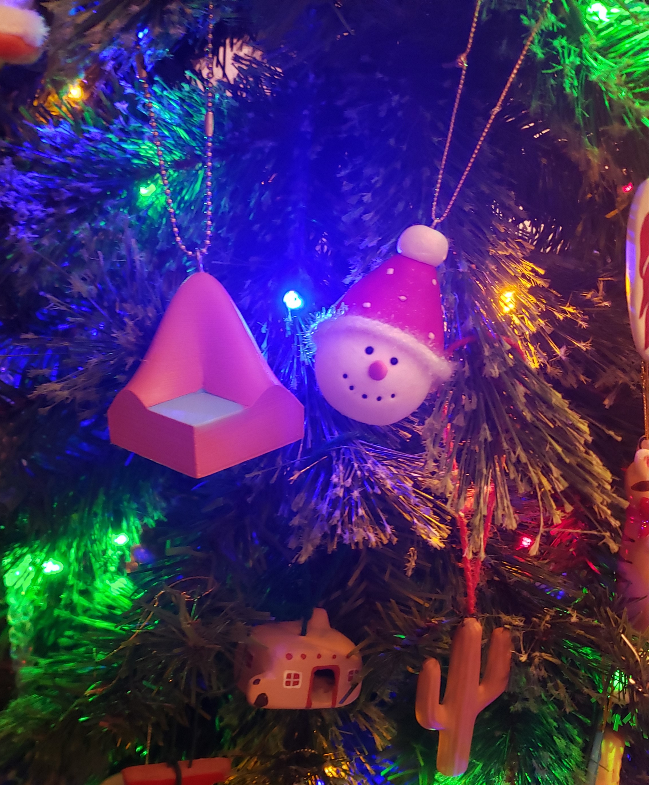
(Sorry - the ornament is not available at the MathWorks Merch Shop -- I made it with a 3-D printer.)
So I made this.
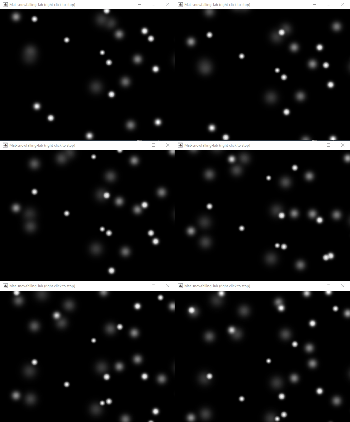
clear
close all
clc
% inspired from: https://www.youtube.com/watch?v=3CuUmy7jX6k
%% user parameters
h = 768;
w = 1024;
N_snowflakes = 50;
%% set figure window
figure(NumberTitle="off", ...
name='Mat-snowfalling-lab (right click to stop)', ...
MenuBar="none")
ax = gca;
ax.XAxisLocation = 'origin';
ax.YAxisLocation = 'origin';
axis equal
axis([0, w, 0, h])
ax.Color = 'k';
ax.XAxis.Visible = 'off';
ax.YAxis.Visible = 'off';
ax.Position = [0, 0, 1, 1];
%% first snowflake
ht = gobjects(1, 1);
for i=1:length(ht)
ht(i) = hgtransform();
ht(i).UserData = snowflake_factory(h, w);
ht(i).Matrix(2, 4) = ht(i).UserData.y;
ht(i).Matrix(1, 4) = ht(i).UserData.x;
im = imagesc(ht(i), ht(i).UserData.img);
im.AlphaData = ht(i).UserData.alpha;
colormap gray
end
%% falling snowflake
tic;
while true
% add a snowflake every 0.3 seconds
if toc > 0.3
if length(ht) < N_snowflakes
ht = [ht; hgtransform()];
ht(end).UserData = snowflake_factory(h, w);
ht(end).Matrix(2, 4) = ht(end).UserData.y;
ht(end).Matrix(1, 4) = ht(end).UserData.x;
im = imagesc(ht(end), ht(end).UserData.img);
im.AlphaData = ht(end).UserData.alpha;
colormap gray
end
tic;
end
ax.CLim = [0, 0.0005]; % prevent from auto clim
% move snowflakes
for i = 1:length(ht)
ht(i).Matrix(2, 4) = ht(i).Matrix(2, 4) + ht(i).UserData.velocity;
end
if strcmp(get(gcf, 'SelectionType'), 'alt')
set(gcf, 'SelectionType', 'normal')
break
end
drawnow
% delete the snowflakes outside the window
for i = length(ht):-1:1
if ht(i).Matrix(2, 4) < -length(ht(i).Children.CData)
delete(ht(i))
ht(i) = [];
end
end
end
%% snowflake factory
function snowflake = snowflake_factory(h, w)
radius = round(rand*h/3 + 10);
sigma = radius/6;
snowflake.velocity = -rand*0.5 - 0.1;
snowflake.x = rand*w;
snowflake.y = h - radius/3;
snowflake.img = fspecial('gaussian', [radius, radius], sigma);
snowflake.alpha = snowflake.img/max(max(snowflake.img));
end
Hello, MATLAB fans!
For years, many of you have expressed interest in getting your hands on some cool MathWorks merchandise. I'm thrilled to announce that the wait is over—the MathWorks Merch Shop is officially open!

In our shop, you'll find a variety of exciting items, including baseball caps, mugs, T-shirts, and YETI bottles.
Visit the shop today and explore all the fantastic merchandise we have to offer. Happy shopping!
We are thrilled to announce the grand prize winners of our MATLAB Shorts Mini Hack contest! This year, we invited the MATLAB Graphics and Charting team, the authors of the MATLAB functions used in every entry, to be our judges. After careful consideration, they have selected the top three winners:
Judge comments: Realism & detailed comments; wowed us with Manta Ray
2nd place – Jenny Bosten
Judge comments: Topical hacks : Auroras & Wind turbine; beautiful landscapes & nightscapes
3rd place - Vasilis Bellos
Judge comments: Nice algorithms & extra comments; can’t go wrong with Pumpkins
Judge comments: Impressive spring & cubes!
In addition, after validating the votes, we are pleased to announce the top 10 participants on the leaderboard:
Congratulations to all! Your creativity and skills have inspired many of us to explore and learn new skills, and make this contest a big success!
Dear MATLAB contest enthusiasts,
Welcome to the third installment of our interview series with top contest participants! This time we had the pleasure of talking to our all-time rock star – @Jenny Bosten. Every one of her entries is a masterpiece, demonstrating a deep understanding of the relationship between mathematics and aesthetics. Even Cleve Moler, the original author of MATLAB, is impressed and wrote in his blog: "Her code for Time Lapse of Lake View to the West shows she is also a wizard of coordinate systems and color maps."
you to read it to learn more about Jenny’s journey, her creative process, and her favorite entries.
Question: Who would you like to see featured in our next interview? Let us know your thoughts in the comments!
It would be nice to have a function to shade between two curves. This is a common question asked on Answers and there are some File Exchange entries on it but it's such a common thing to want to do I think there should be a built in function for it. I'm thinking of something like
plotsWithShading(x1, y1, 'r-', x2, y2, 'b-', 'ShadingColor', [.7, .5, .3], 'Opacity', 0.5);
So we can specify the coordinates of the two curves, and the shading color to be used, and its opacity, and it would shade the region between the two curves where the x ranges overlap. Other options should also be accepted, like line with, line style, markers or not, etc. Perhaps all those options could be put into a structure as fields, like
plotsWithShading(x1, y1, options1, x2, y2, options2, 'ShadingColor', [.7, .5, .3], 'Opacity', 0.5);
the shading options could also (optionally) be a structure. I know it can be done with a series of other functions like patch or fill, but it's kind of tricky and not obvious as we can see from the number of questions about how to do it.
Does anyone else think this would be a convenient function to add?
My favorite image processing book is The Image Processing Handbook by John Russ. It shows a wide variety of examples of algorithms from a wide variety of image sources and techniques. It's light on math so it's easy to read. You can find both hardcover and eBooks on Amazon.com Image Processing Handbook
There is also a Book by Steve Eddins, former leader of the image processing team at Mathworks. Has MATLAB code with it. Digital Image Processing Using MATLAB
You might also want to look at the free online book http://szeliski.org/Book/
Over the past 4 weeks, 250+ creative short movies have been crafted. We had a lot of fun and, more importantly, learned new skills from each other! Now it’s time to announce week 4 winners.
Nature:
3D:
Seamless loop:
Holiday:
Fractal:
Congratulations! Each of you won your choice of a T-shirt, a hat, or a coffee mug. We will contact you after the contest ends.
Weekly Special Prizes
Thank you for sharing your tips & tricks with the community. These great technical articles will benefit community users for many years. You won a limited-edition pair of MATLAB Shorts!
In week 5, let’s take a moment to sit back, explore all of the interesting entries, and cast your votes. Reflect what you have learned or which entries you like most. Share anything in our Discussions area! There is still time to win our limited-edition MATLAB Shorts.
In the past two years, large language models have brought us significant changes, leading to the emergence of programming tools such as GitHub Copilot, Tabnine, Kite, CodeGPT, Replit, Cursor, and many others. Most of these tools support code writing by providing auto-completion, prompts, and suggestions, and they can be easily integrated with various IDEs.
As far as I know, aside from the MATLAB-VSCode/MatGPT plugin, MATLAB lacks such AI assistant plugins for its native MATLAB-Desktop, although it can leverage other third-party plugins for intelligent programming assistance. There is hope for a native tool of this kind to be built-in.
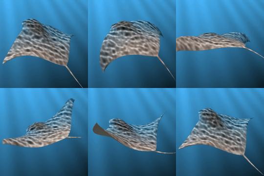
What incredible short movies can be crafted with no more than 2000 characters of MATLAB code? Discover the creativity in our GALLERY from the MATLAB Shorts Mini Hack contest.
Vote on your favorite short movies by Nov.10th. We are giving out MATLAB T-shirts to 10 lucky voters!
Tips: the more you vote, the higher your chance to win.

