The Symbolic Math Toolbox does not have its own dot and and cross functions. That's o.k. (maybe) for garden variety vectors of sym objects where those operations get shipped off to the base Matlab functions
x = sym('x',[3,1]); y = sym('y',[3,1]);
which dot(x,y)
/MATLAB/toolbox/matlab/specfun/dot.m
dot(x,y)
ans = 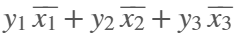
which cross(x,y)
/MATLAB/toolbox/matlab/specfun/cross.m
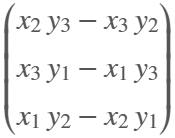
cross(x,y)
ans =
But now we have symmatrix et. al., and things don't work as nicely x = symmatrix('x',[3,1]); y = symmatrix('y',[3,1]);
z = symmatrix('z',[1,1]);
sympref('AbbreviateOutput',false);
dot() expands the result, which isn't really desirable for exposition.
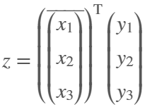
eqn = z == dot(x,y)
eqn =
Also, dot() returns the the result in terms of the conjugate of x, which can't be simplifed away at the symmatrix level
assumeAlso(sym(x),'real')
eqn = z == simplify(dot(x,y))
end
ans = 'Undefined function 'simplify' for input arguments of type 'symmatrix'.'
To get rid of the conjugate, we have to resort to sym
eqn = simplify(sym(eqn))
eqn = 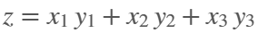
but again we are in expanded form, which defeats the purpose of symmatrix (et. al.)
But at least we can do this to get a nice equation
eqn = z == x.'*y
eqn = 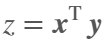
dot errors with symfunmatrix inputs
x = symfunmatrix('x(t)',t,[3,1]); y = symfunmatrix('y(t)',t,[3,1]);
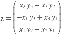
Cross works (accidentally IMO) with symmatrix, but expands the result, which isn't really desirable for exposition
x = symmatrix('x',[3,1]); y = symmatrix('y',[3,1]);
z = symmatrix('z',[3,1]);
eqn = z == cross(x,y)
eqn =
w = symfunmatrix('w(t)',t,[3,1]);
end
ans = 'A and B must be of length 3 in the dimension in which the cross product is taken.'
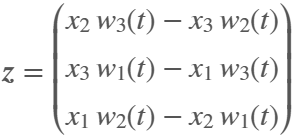
In the latter case we can expand with
eqn = z == cross(sym(x),symfun(w))
eqn(t) =
But we can't do the same with dot (as shown above, dot doesn't like symfun inputs)
eqn = z == dot(sym(x),symfun(w))
Looks like the only choice for dot with symfunmatrix is to write it by hand at the matrix level
x.'*w
ans(t) = 
or at the sym/symfun level
sym(x).'*symfun(w)
ans(t) = 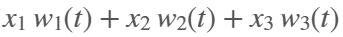
Ideally, I'd like to see dot and cross implemented for symmatrix and symfunmatrix types where neither function would evaluate, i.e., expand, until both arguments are subs-ed with sym or symfun objects of appropriate dimension.
Also, it would be nice if symmatrix could be assumed to be real. Is there a reason why being able to do so wouldn't make sense?
end
ans = 'Undefined function 'assume' for input arguments of type 'symmatrix'.'