Analysis of Inset-Feed Patch Antenna on Dielectric Substrate
This example showcases the analysis of an inset-feed patch antenna on a low-epsilon, low-loss, thin dielectric substrate. The results are compared with the reflection coefficient and surface currents around the 2.4 GHz, Wi-Fi band for a reference design [1]. The Antenna Toolbox™ library of antenna elements includes a patch antenna model that is driven with a coaxial probe. Another way to excite the patch is by using an inset-feed. The inset-feed is a simple way to excite the patch and allows for planar feeding techniques such as a microstrip line.
Inset-Feed Patch Antenna
The inset-feed patch antenna typically comprises of a notch that is cut from the non-radiating edge of the patch to allow for the planar feeding mechanism. Typical feeding mechanism involves a microstrip line coplanar with the patch. The notch size, i.e. the length and the width are calculated to achieve an impedance match at the operating frequency. A common analytical expression that is used to determine the inset feed position , the distance from the edge of the patch along its length, is shown below [2]. The patch length and width are L, W respectively.
It is also common to excite the patch along the center line (y = W/2), where W is the width of the patch antenna, which makes the y-coordinate zero. This is the reason, the expression shown above, is only in terms of the x-coordinate.
Create Geometry and Mesh
The PDE toolbox™ has been used to create the geometry and mesh the structure. Use the triangulation function in MATLAB™ to visualize the mesh.
load insetfeedpatchmesh
T = triangulation(t(1:3,:)',p');
figure
triplot(T)
axis equal
grid on
xlabel('x')
ylabel('y')

Create Patch Antenna
Use the customAntennaMesh from Antenna Toolbox™ to transform this mesh into an antenna. Use the createFeed function to define the feed.
c = customAntennaMesh(p,t);
createFeed(c,[-0.045 0 0],[-0.0436 0 0])
show(c)
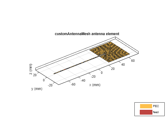
A note about the feeding point on the microstrip line* The feed point chosen is such that it is from the open circuit end of the line [3]. In addition a relatively long line length is chosen to facilitate an accurate calculation of the s-parameters. The wavelength in the dielectric is approximated relative to the wavelength in free-space as
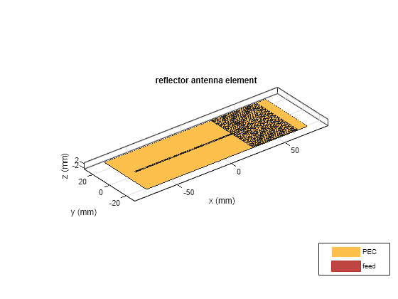
Provide groundplane backing to radiator Patch antennas are backed by a ground plane. Do this by assigning the customAntennaMesh as an exciter for a reflector.
r = reflector;
r.Exciter = c;
r.GroundPlaneLength = 15e-2;
r.GroundPlaneWidth = 5e-2;
r.Spacing = 0.381e-3;
show(r)
Assign Substrate to Patch Antenna
Define a dielectric material with and loss tangent of 0.0009. Assign this dielectric material to the Substrate property in the reflector.
d = dielectric;
d.Name = 'RT5880';
d.EpsilonR = 2.2;
d.LossTangent = 0.0009;
r.Substrate = d;
show(r)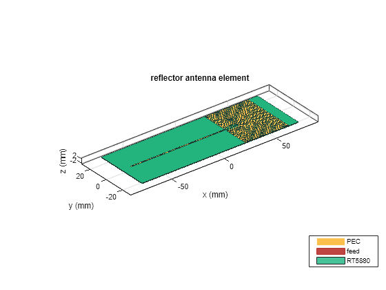
Analysis of Patch Antenna
The overall dimensions of this patch antenna are large and therefore will result in a relatively large mesh (dielectric + metal). The structure is analyzed by meshing it with a maximum edge length of 4 mm and solved for the scattering parameters. The maximum edge length was chosen to be slightly less than the default maximum edge length computed at the highest frequency in the analysis range of 2.45 GHz, which is about 4.7 mm. The analyzed antennas are loaded from a MAT file to the workspace.
load insetfeedpatchCalculate S-Parameters of Patch Antenna
The center frequency of analysis is approximately 2.4 GHz. Define the frequency range
freq = linspace(2.35e9,2.45e9,41);
s = sparameters(r,freq,50);
figure
rfplot(s,1,1)

The plot shows the expected dip in the reflection coefficient close to 2. 4 GHz. The default reference impedance is set to 50 . Use the -10 dB criterion to determine the reflection coefficient bandwidth for this patch to be less than 1%.
Visualize Current Distribution
Use the function current, to plot the surface current distribution for this patch antenna at approximately 2.4 GHz. The current is minimum at the edges along its length and maximum in the middle.
figure
current(r,2.4e9)
view(0,90)

Discussion
The results for this patch antenna are in good agreement with the reference results reported in [1], pg.111 - 114.
Reference
[1] Jagath Kumara Halpe Gamage,"Efficient Space Domain Method of Moments for Large Arbitrary Scatterers in Planar Stratified Media", Dept. of Electronics and Telecommunications, Norwegian University of Science and Technology.
[2] Lorena I. Basilio, M. A. Khayat, J. T. Williams, S. A. Long, "The dependence of the input impedance on feed position of probe and microstrip line-fed patch antennas," IEEE Transactions on in Antennas and Propagation, vol. 49, no. 1, pp.45-47, Jan 2001.
[3] P. B. Katehi and N. G. Alexopoulos, "Frequency-dependent characteristics of microstrip discontinuities in millimeter wave integrated circuits," IEEE Transactions on Microwave Theory and Techniques, vol. 33, no. 10, pp. 1029-1035, 1985.