Audio-Based Anomaly Detection for Machine Health Monitoring

This example shows how to design an autoencoder neural network to perform anomaly detection for machine sounds using unsupervised learning. In this example you will download and process the data using a log-mel spectrogram, design and train an autoencoder network, and make out-of-sample predictions by applying a statistical model to the trained network output.
Audio-based anomaly detection is the process of identifying whether the sound generated by an object is abnormal. This is applicable to the automatic detection of industrial component failures, as a machine that emits an abnormal sound is likely malfunctioning.
The problem of classifying sounds as either normal or abnormal can be viewed as a standard supervised learning task, where a model is trained on samples of both sound types and learns to discriminate between them. However, in practice, a data set of abnormal sounds is generally not available because machine malfunctions do not occur frequently enough or for long enough duration to be properly recorded. Also, it would be impossible to create a data set representative of every type of anomaly, as a machine could malfunction for a diverse set of reasons.
Autoencoders are useful for anomaly detection tasks because they train solely on the normal samples. Autoencoder networks perform the unsupervised learning task of finding both a low-dimensional encoding of the input as well as a rule to accurately reconstruct the input from its low-dimensional representation. This forces the autoencoder to learn a process specifically for compressing and decompressing normal samples. The motivating principle is that when an abnormal sample is fed into the autoencoder, the reconstruction error will be much larger than expected from the training set because the signal compression and decompression scheme learned by the network is only expected to work well for normal samples. To make predictions on unseen samples, an error threshold is picked based off the expected distribution of reconstruction errors for normal samples, and any input with an error larger than the threshold is classified as an anomaly.
In this example, the autoencoder first passes the input through an encoding section of fully-connected layers using a number of nodes on the same order of magnitude as the input dimension. The data then feeds into a bottleneck layer with a number of nodes much smaller than the input size which forces the network to compress the input signal into the lower-dimensional representation. This compressed representation feeds into a decoding section that generally mirrors the same architecture as the encoder section in order to recreate the input signal. Lastly, the decoder output is passed into a final output layer with the same number of dimensions as the input. The network loss is taken as the regression error between the original input and the reconstructed signal.
Download Data
This example applies to the second task of the Detection and Classification of Acoustic Scenes and Events (DCASE) 2022 challenge [1]. The example uses a subset of the public data set from Sound Dataset for Malfunctioning Industrial Machine Investigation and Inspection [2] to train and evaluate the autoencoder. It implements ideas from the preprocessing steps and network designs of both the autoencoder baseline system in [1] and the proposed network in [2] and uses the performance metrics devised in [1] to analyze the testing results.
Download a subset of the data set in [2] that contains recorded audio files of 4 different fan types, labeled by ID number. There are both normal and abnormal recordings for each fan type. These files contain 1 channel sampled at 16 kHz and are 10 seconds long. The samples are recordings of operating fans with background noise with a signal to noise ratio of 6 dB. A full explanation of the data collection process is available in [2].
dataFolder = tempdir;
dataset = fullfile(dataFolder,"fan6db");
supportFileLoc = "mimii/mono/fan6db.zip";
downloadFolder = matlab.internal.examples.downloadSupportFile("audio",supportFileLoc);
unzip(downloadFolder,dataFolder)
Investigate Data
To briefly examine the data set and the differences between the normal and abnormal recordings, select one recording of each type from the ID 00 fan data set and play the first two seconds over your speaker.
[normalSample,fs] = audioread(fullfile(dataset,"id_00","normal_00","00000000.wav"));
abnormalSample = audioread(fullfile(dataset,"id_00","abnormal_00","00000000.wav"));

numSamples = 10*fs;

sound(normalSample(1:numSamples/5),fs)
pause(3)
sound(abnormalSample(1:numSamples/5),fs)
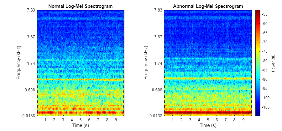
Both recordings are dominated by a single tone, and this tone is clearly higher pitched in the abnormal sample.
Preprocess Data
You can optionally set the speedUp flag to true to reduce the size of the data set used in the example. If you set this to true you can quickly verify that the script runs as expected, but the results will be skewed.
speedUp =  false;
Separate the data set into two audioDatastore objects, one with the normal samples and one with the abnormal samples. Since the autoencoder only trains on the normal samples, hold out the abnormal samples to be included in the test set.
ads = audioDatastore(dataset, ...
    IncludeSubfolders=true, ...
    LabelSource="foldernames", ...
    FileExtensions=".wav");

normalLabels = categorical(["normal_00","normal_02","normal_04","normal_06"]);
abnormalLabels = categorical(["abnormal_00","abnormal_02","abnormal_04","abnormal_06"]);

isNormal = ismember(ads.Labels,normalLabels);
isAbnormal = ~isNormal;
adsNormal = subset(ads,isNormal);
adsTestAbnormal = subset(ads,isAbnormal);
rng(3);
if speedUp
    c = cvpartition(adsTestAbnormal.Labels,kFold=8,Stratify=true);
    adsTestAbnormal = subset(adsTestAbnormal,c.test(1));
end
Divide the normal samples into training, validation, and test sets, stratified by ID number. Then concatenate the normal test set with the abnormal samples to form the full test set.
c = cvpartition(adsNormal.Labels,kFold=8,Stratify=true);
if speedUp
    trainInd = c.test(3);
else
    trainInd = ~boolean(c.test(1)+c.test(2));
end
valInd = c.test(1);
testInd = c.test(2);

adsTrain = subset(adsNormal,trainInd);
adsVal = subset(adsNormal,valInd);
adsTestNormal = subset(adsNormal,testInd);
Transform each of the datastores by applying an STFT with frame length of 64 ms and hop length of 32 ms, find the log-mel energies for 128 frequency bands, and then concatenate these frames into overlapping, consecutive groups of 5 to form a context window. It is common to use log-mel energies as inputs to audio deep learning tasks as they represent the spectrum of tones on a scale similar to how humans perceive sound. Visualize the log-mel spectrograms of the two clips played previously using the plotLogMelSpect supporting function.
plotLogMelSpect(normalSample,abnormalSample);
Use the processData supporting function to perform the data transformation.
tdsTrain = transform(adsTrain,@processData);
tdsVal = transform(adsVal,@processData);
tdsTestNormal = transform(adsTestNormal,@processData);
tdsTestAbnormal = transform(adsTestAbnormal,@processData);
Read the data into arrays where each column represents an input sample. Do this in parallel if you have enabled Parallel Computing Toolbox™. Then combine the normal test set and abnormal data set into the full test set, and label the samples accordingly.
trainingData = readall(tdsTrain,UseParallel=false);
valData = readall(tdsVal,UseParallel=canUseParallelPool);

normalTestData = readall(tdsTestNormal,UseParallel=canUseParallelPool);
abnormalTestData = readall(tdsTestAbnormal,UseParallel=canUseParallelPool);
testLabels = categorical([zeros(length(adsTestNormal.Labels),1);ones(length(adsTestAbnormal.Labels),1)],[0,1],["normal","abnormal"]);
testData = [normalTestData;abnormalTestData];
Network Architecture
The encoder section consists of 2 fully connected layers with output sizes of 128. The bottleneck layer constrains the network to an 8-dimensional representation of the original 640-dimensional input. The decoder section mirrors the encoder architecture as the input is reconstructed and fed into the output layer. Use half-mean-squared-error as the loss function to train the network and quantify the reconstruction error.
layers = [

featureInputLayer(640)

fullyConnectedLayer(128,Name="Encoder1")
batchNormalizationLayer
reluLayer

fullyConnectedLayer(128,Name="Encoder2")
batchNormalizationLayer
reluLayer

fullyConnectedLayer(8,Name="Bottleneck")
batchNormalizationLayer
reluLayer

fullyConnectedLayer(128,Name="Decoder1")
batchNormalizationLayer
reluLayer

fullyConnectedLayer(128,Name="Decoder2")
batchNormalizationLayer
reluLayer

fullyConnectedLayer(640,Name="Output")];
Train Network
Train the network using an ADAM optimizer for 40 epochs. Shuffle the mini-batches each epoch, and set the ExecutionEnvironment field to "auto" so that a GPU is used instead of the CPU if available. If using a GPU with limited memory, you may need to decrease the value of the miniBatchSize field. The training parameter settings were found empirically to optimize convergence speed. This may take 10-15 minutes depending on your hardware.
batchSize = length(trainingData)/4;
if speedUp
    batchSize = 2*batchSize;
end

options = trainingOptions("adam", ...
    MaxEpochs=30, ...
    InitialLearnRate=1e-2, ...
    LearnRateSchedule="piecewise", ...
    LearnRateDropPeriod=5, ...
    LearnRateDropFactor=0.7, ...
    GradientDecayFactor=0.8, ...
    miniBatchSize=batchSize, ...
    Shuffle="every-epoch", ...
    ExecutionEnvironment="auto", ...
    ValidationData={valData,valData}, ...
    ValidationFrequency=16, ...
    Verbose=false, ...
    Plots="training-progress");
trainingData is both the input and the target output as the network attempts to regress the training data on itself with the low-dimensional encoding constraint. Your results should look similar to the training plots below.
[net,info] = trainnet(trainingData,trainingData,layers,"mse",options);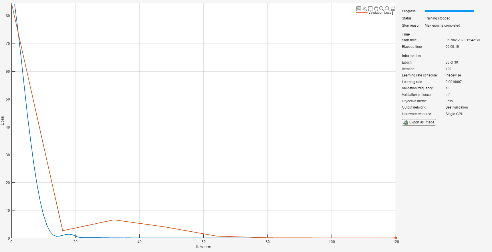
Evaluate Performance
For each input to the network, the autoencoder outputs an attempted reconstruction. However, each network input is only one context window from a larger audio sample. For each of these network inputs, the error is defined as the squared L-2 norm of the difference between the original input and the network output. To calculate a decision metric for each entire audio sample, the errors for each context window associated with that audio sample are added together, and this sum is divided by the product of the network input dimension and the number of context groups per audio sample. For an audio sample , the decision function metric is denoted and defined where is the number of context groups per sample, is the context group constructed from , and is the network output for . represents the mean squared reconstruction error across each vector component of all context windows associated with an audio sample .
For each input , can also be interpreted as a relative measure of the network's confidence that is abnormal, with higher values indicating larger confidence. To deploy this model and make predictions on new data, you must select a decision boundary on the values of to separate positive and negative predictions. Model for normal samples as a gamma distribution. Gamma distributions are commonly used to model autoencoder reconstruction errors since the errors are usually skewed right with a heavy tail, which is the natural shape of a gamma distribution. In this example, the decision boundary is selected as the point that corresponds to an expected false positive rate (FPR) p = 0.1. This decision boundary attempts to capture all truly abnormal samples while tolerating the expectation that 10% of normal samples will be falsely predicted as abnormal. You can choose a specific value of p to fit your individual system constraints.
p = 0.1;
Compute the values of over the training set and store them in the variable A_train using the helper function getScore. Then solve for the maximum likelihood estimate for the gamma distribution parameters, select the cutoff point from the inverse gamma cumulative distribution function, and plot the fitted distribution with the histogram of using the getCutoff helper function.
trainRecons = minibatchpredict(net,trainingData,MiniBatchSize=size(trainingData,1)/4);
A_train = getScore(trainingData,trainRecons);
cutoff = getCutoff(A_train,p);

Verify that this cutoff point roughly corresponds to an FPR of 0.1 on the training set:
sum(A_train > cutoff) / length(A_train)
ans = 0.1221
Test the classification accuracy of this system with the chosen cutoff point on the holdout test set.
testRecons = minibatchpredict(net,testData,MiniBatchSize=size(testData,1));
A_test = getScore(testData,testRecons);
testPreds = categorical(A_test > cutoff,[false,true],["normal","abnormal"]).';
figure
cm = confusionchart(testLabels,testPreds);
cm.RowSummary="row-normalized";
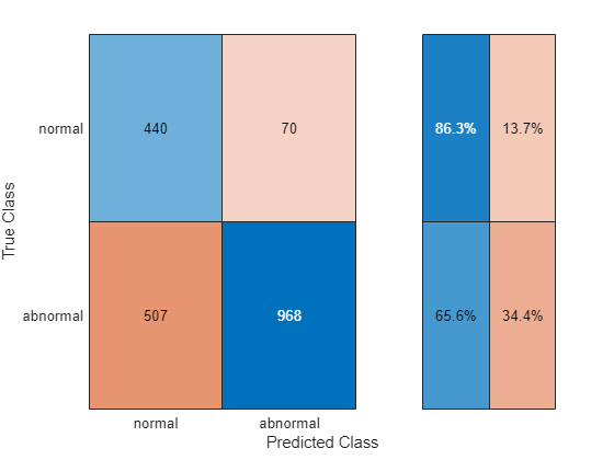
Using this cutoff point, the model achieves a true positive rate (TPR) of 0.647 at the cost of an FPR of 0.125.
To evaluate the accuracy of the network over a range of decision boundaries, measure the overall performance on the test set by the area under the receiver operating characteristic curve (AUC). Use both the full AUC and the partial AUC (pAUC) to analyze the network performance. pAUC is the AUC on the subdomain where the FPR is on the interval divided by the maximum possible area in the interval, which is p. It is important to consider pAUC since anomaly detection systems need to be able to achieve high TPR while keeping the FPR to a minimum, as a system with frequent false alarms is untrustworthy and unusable. Compute the AUC using the perfcurve function from Statistics and Machine Learning Toolbox™.
[X,Y,T,AUC] = perfcurve(testLabels,A_test,categorical("abnormal"));
[~,cutoffIdx] = min(abs(T-cutoff));

figure
plot(X,Y);
xlabel("FPR");
ylabel("TPR");
title("Test Set ROC Curve");
hold on
plot(X(cutoffIdx),Y(cutoffIdx),'r*');
hold off
legend("ROC Curve","Cutoff Decision Point");
grid on
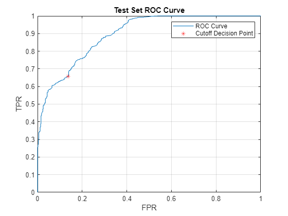
AUC
AUC = single
    0.8949
To calculate the pAUC, approximate the area under the curve in the first tenth of the FPR domain using trapz. For reference, the expected value of the pAUC of a random classifier is 0.05.
pX = X(X <= p);
pY = Y(X <= p);
pAUC = trapz(pX,pY)/p
pAUC = single
    0.5177
The network separates the normal and abnormal test samples fairly well and is able to learn a single encoding across multiple fan IDs. Visualize the difference in reconstruction errors between the normal and abnormal groups by their histograms.
figure
hold on
edges = linspace(min(A_test),1,100);
histogram(A_test(testLabels == categorical("normal")),edges,Normalization="probability");
histogram(A_test(testLabels == categorical("abnormal")),edges,Normalization="probability");
ylabel("Sample Probability");
xlabel("Reconstruction Error (A)");
legend("Normal","Abnormal");
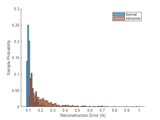
Although there is some overlap, the distribution of reconstruction errors for the abnormal samples is offset further to the right and contains a much heavier tail than the distribution of reconstruction errors over the normal samples.
Lastly, evaluate the model's performance on each fan ID individually to reveal any imbalance between the fan types and check if the model is able to predict universally well over all IDs.
IDs = [0;2;4;6];
AUCs = zeros(4,1);
pAUCs = AUCs;
A_testNormal = A_test(1:sum(testInd));
A_testAbnormal = A_test(sum(testInd)+1:end);
for ii = 1:4
    normalMask = adsTestNormal.Labels == normalLabels(ii);
    abnormalMask = adsTestAbnormal.Labels == abnormalLabels(ii);
    A_testByID = [A_testNormal(normalMask) A_testAbnormal(abnormalMask)];
    testLabelsByID = [adsTestNormal.Labels(normalMask);adsTestAbnormal.Labels(abnormalMask)];
    [X_ID,Y_ID,T_ID,AUC_ID] = perfcurve(testLabelsByID,A_testByID,abnormalLabels(ii));
    AUCs(ii) = AUC_ID;
    pX_ID = X_ID(X_ID <= p);
    pY_ID = Y_ID(X_ID <= p);
    pAUCs(ii) = trapz(pX_ID,pY_ID)/p;
end
disp(table(IDs,AUCs,pAUCs));
    IDs     AUCs       pAUCs
    ___    _______    _______

     0     0.72849     0.1776
     2     0.96949      0.683
     4     0.90909    0.47002
     6     0.95452    0.67158
The results show the model performance significantly varies by fan type. This result is important to note as this network is relatively small and simple compared to the top performing DCASE challenge submissions in [3]. To generalize better across fan types and to different domains, a more complex model is needed. However, if you know the exact fan type that you are deploying an anomaly detector for, a very light-weight model like the one in this example may suffice.
Supporting Functions
function plotLogMelSpect(normalSample,abnormalSample)
%PLOTLOGMELSPECT plots the log-mel spectrogram of the normal and abornomal
%   plotLogMelSpect(normalSample,abnormalSample) plots the log-mel
%   spectrogram of the two inputs side by side, with parameters consistent
%   with the data preprocessing transformation used to prepare the signals
%   to be fed into the autoencoder.
f = figure;
f.Position(3) = 900;
samples = {normalSample,abnormalSample};
fs = 16e3;
winDur = 64e-3;
winLen = winDur * fs;
numMelBands = 128;
tiledlayout(1,2)
for i = 1:2
    nexttile
    x = samples{i};
    melSpectrogram(x,fs,Window=hamming(winLen,"periodic"),FFTLength=winLen,OverlapLength=winLen/2,NumBands=numMelBands);
    xticks(1:10);
    xticklabels(string(1:10));
    colormap("jet");
    if i == 2
        cbar = colorbar;
        cbar.Label.String = "Power (dB)";
        title("Abnormal Log-Mel Spectrogram");
        ylabel([]);
    else
        colorbar off
        title("Normal Log-Mel Spectrogram");
    end
end
end
function features = processData(x)
%PROCESSDATA transforms an audio file input x into the autoencoder network
%input format
%   features = processData(x) takes the STFT of audio data x, transforms
%   the STFT into the log-mel spectrogram, and then constructs context
%   groups of consecutive mel-spectrogram frames. The function returns the
%   features as a numContextGroupsPerSample-by-contextGroupSize matrix. For
%   this data set, numContextGroupsPerSample = 309 and contextGroupSize =
%   640 = 128*5 (since there are 128 mel bands per frame and 5 frames are
%   concatenated for each context group)

fs = 16e3;
winDur = 64e-3;
winLen = winDur*fs;
numMelBands = 128;
afe = audioFeatureExtractor(...
    Window=hamming(winLen,"periodic"), ...
    FFTLength=winLen, ...
    OverlapLength=winLen/2, ...
    SampleRate=fs, ...
    melSpectrum=true);
setExtractorParameters(afe,"melSpectrum",numBands=numMelBands,ApplyLog=true);

% Zero pad
numPad = numel(x) + winLen - mod(numel(x),winLen);
xPadded = resize(x,numPad,Side="both");

% Extract
features = {extract(afe,xPadded)};
features = cellfun(@groupSTFT,features,UniformOutput=false);
features = cat(1,features{:});
end

function groups = groupSTFT(x)
%GROUPSTFT transforms an STFT x into context groups of size 5
%   groups = groupSTFT(x) transforms the STFT x by grouping each STFT frame
%   with the following 4 frames to form context groups of size 5. This
%   creates multiple network inputs out of each audio sample, each of size
%   contextLen*numMelBands = 5*128 = 640. Each of these context groups are
%   treated as individual 640-dimensional vectors for the purpose of the
%   autoencoder.
contextLen = 5;
numMelBands = 128;
x_flat = reshape(x',1,[]);
groups = buffer(x_flat,contextLen*numMelBands,numMelBands*(contextLen-1),"nodelay")';
end

function A = getScore(data,preds)
%GETSCORE returns the reconstruction error for each sample in data
%   A = getScore(data,preds) returns A(X) for each X in the set of samples
%   transformed into network input data.
err = sum((preds-data).^2,2);
numSTFTFrames = 313;
contextWin = 5;
numMelFilters = 128;
numContextGroupsPerSample = numSTFTFrames - contextWin + 1;
numSamples = length(err)/numContextGroupsPerSample;
A_total = reshape(err,[numContextGroupsPerSample,numSamples]); %Each column contains reconstruction errors of all context groups for one sample
A = sum(A_total)/(numMelFilters*contextWin*numSTFTFrames); %Each entry is a reconstruction error for each sample
end

function cutoff = getCutoff(A,p)
%GETCUTOFF fits a gamma distribution to A and returns the cutoff as the inverse cdf of 1-p
%   cutoff = getCutoff(A,p) fits a gamma distribution to the reconstruction
%   error array A, solves for the cutoff point as the inverse gamma cdf
%   evaluated at 1-p, and plots the fitted distribution along with the
%   histogram of A and the calculated cutoff point. A is expected as
%   one-by-numSamples array where numSamples is the number of audio samples
%   used to compute the reconstruction error values of A.
gammaParams = gamfit(A);
a = gammaParams(1);
b = gammaParams(2);
cutoff = gaminv(1-p,a,b);
figure
ax1 = subplot(4,1,1:3);
histogram(A);
xticks([]);
title("Histogram of A with Fitted Gamma Dist. PDF");
ylTop = ylabel("Count");
xline(cutoff,"--",LineWidth=2,Label="cutoff",LabelOrientation="horizontal",LabelVerticalAlignment="middle");
ax2 = subplot(4,1,4);
t = linspace(0, max(A), 1000);
y = gampdf(t,a,b);
plot(t,y);
xline(cutoff,"--",LineWidth=2);
ylBottom = ylabel("\Gamma Density");
yticks([]);
linkaxes([ax1 ax2],"x");
ylBottom.Position(1) = ylTop.Position(1);
xlabel("Reconstruction Error (A)");
xlim([0 .4]);
ylBottom.Position(1) = ylTop.Position(1);
end
References
[1] "Unsupervised anomalous sound detection for machine condition monitoring applying domain generalization techniques," DCASE 2022. [Online]. Available: https://dcase.community/challenge2022/task-unsupervised-anomalous-sound-detection-for-machine-condition-monitoring. [Accessed: 08-Jun-2022].
[2] "Purohit, Harsh, Tanabe, Ryo, Ichige, Kenji, Endo, Takashi, Nikaido, Yuki, Suefusa, Kaori, & Kawaguchi, Yohei. (2019). MIMII Dataset: Sound Dataset for Malfunctioning Industrial Machine Investigation and Inspection (public 1.0) [Data set]. 4th Workshop on Detection and Classification of Acoustic Scenes and Events (DCASE 2019 Workshop), New York, USA. Zenodo. https://doi.org/10.5281/zenodo.3384388. Dataset is licensed under the Creative Commons Attribution-ShareAlike 4.0 International License available at https://creativecommons.org/licenses/by-sa/4.0/
[3] "Unsupervised detection of anomalous sounds for Machine Condition Monitoring," DCASE 2020. [Online]. Available: https://dcase.community/challenge2020/task-unsupervised-detection-of-anomalous-sounds-results#Giri2020. [Accessed: 08-Jun-2022].