Detecting DNA Copy Number Alteration in Array-Based CGH Data
This example shows how to detect DNA copy number alterations in genome-wide array-based comparative genomic hybridization (CGH) data.
Introduction
Copy number changes or alterations is a form of genetic variation in the human genome [1]. DNA copy number alterations (CNAs) have been linked to the development and progression of cancer and many diseases.
DNA microarray based comparative genomic hybridization (CGH) is a technique allows simultaneous monitoring of copy number of thousands of genes throughout the genome [2,3]. In this technique, DNA fragments or "clones" from a test sample and a reference sample differentially labeled with dyes (typically, Cy3 and Cy5) are hybridized to mapped DNA microarrays and imaged. Copy number alterations are related to the Cy3 and Cy5 fluorescence intensity ratio of the targets hybridized to each probe on a microarray. Clones with normalized test intensities significantly greater than reference intensities indicate copy number gains in the test sample at those positions. Similarly, significantly lower intensities in the test sample are signs of copy number loss. BAC (bacterial artificial chromosome) clone based CGH arrays have a resolution in the order of one million base pairs (1Mb) [3]. Oligonucleotide and cDNA arrays provide a higher resolution of 50-100kb [2].
Array CGH log2-based intensity ratios provide useful information about genome-wide CNAs. In humans, the normal DNA copy number is two for all the autosomes. In an ideal situation, the normal clones would correspond to a log2 ratio of zero. The log2 intensity ratios of a single copy loss would be -1, and a single copy gain would be 0.58. The goal is to effectively identify locations of gains or losses of DNA copy number.
The data in this example is the Coriell cell line BAC array CGH data analyzed by Snijders et al.(2001). The Coriell cell line data is widely regarded as a "gold standard" data set. You can download this data of normalized log2-based intensity ratios and the supplemental table of known karyotypes from https://www.nature.com/articles/ng754#supplementary-information. You will compare these cytogenically mapped alterations with the locations of gains or losses identified with various functions of MATLAB and its toolboxes.
For this example, the Coriell cell line data are provided in a MAT file. The data file coriell_baccgh.mat contains coriell_data, a structure containing of the normalized average of the log2-based test to reference intensity ratios of 15 fibroblast cell lines and their genomic positions. The BAC targets are ordered by genome position beginning at 1p and ending at Xq.
load coriell_baccgh
coriell_data
coriell_data =

  struct with fields:

             Sample: {1×15 cell}
         Chromosome: [2285×1 int8]
    GenomicPosition: [2285×1 int32]
          Log2Ratio: [2285×15 double]
            FISHMap: {2285×1 cell}
Visualizing the Genome Profile of the Array CGH Data Set
You can plot the genome wide log2-based test/reference intensity ratios of DNA clones. In this example, you will display the log2 intensity ratios for cell line GM03576 for chromosomes 1 through 23.
Find the sample index for the CM03576 cell line.
sample = find(strcmpi(coriell_data.Sample, 'GM03576'))
sample =

     8
To label chromosomes and draw the chromosome borders, you need to find the number of data points of in each chromosome.
chr_nums = zeros(1, 23);
chr_data_len = zeros(1,23);
for c = 1:23
    tmp = coriell_data.Chromosome == c;
    chr_nums(c) = find(tmp, 1, 'last');
    chr_data_len(c) = length(find(tmp));
end

% Draw a vertical bar at the end of a chromosome to indicate the border
x_vbar = repmat(chr_nums, 3, 1);
y_vbar = repmat([2;-2;NaN], 1, 23);

% Label the autosomes with their chromosome numbers, and the sex chromosome
% with X.
x_label = chr_nums - ceil(chr_data_len/2);
y_label = zeros(1, length(x_label)) - 1.6;
chr_labels = num2str((1:1:23)');
chr_labels = cellstr(chr_labels);
chr_labels{end} = 'X';

figure
hold on
h_ratio = plot(coriell_data.Log2Ratio(:,sample), '.');
h_vbar = line(x_vbar, y_vbar, 'color', [0.8 0.8 0.8]);
h_text = text(x_label, y_label, chr_labels,...
             'fontsize', 8, 'HorizontalAlignment', 'center');

h_axis = h_ratio.Parent;
h_axis.XTick = [];
h_axis.YGrid = 'on';
h_axis.Box = 'on';
xlim([0 chr_nums(23)])
ylim([-1.5 1.5])

title(coriell_data.Sample{sample})
xlabel({'', 'Chromosome'})
ylabel('Log2(T/R)')
hold off

In the plot, borders between chromosomes are indicated by grey vertical bars. The plot indicates that the GM03576 cell line is trisomic for chromosomes 2 and 21 [3].
You can also plot the profile of each chromosome in a genome. In this example, you will display the log2 intensity ratios for each chromosome in cell line GM05296 individually.
sample = find(strcmpi(coriell_data.Sample, 'GM05296'));
figure;
for c = 1:23
    idx = coriell_data.Chromosome == c;
    chr_y = coriell_data.Log2Ratio(idx, sample);
    subplot(5,5,c);

    hp = plot(chr_y, '.');
    line([0, chr_data_len(c)], [0,0], 'color', 'r');

    h_axis = hp.Parent;
    h_axis.XTick = [];
    h_axis.Box = 'on';
    xlim([0 chr_data_len(c)])
    ylim([-1.5 1.5])
    xlabel(['chr ' chr_labels{c}], 'FontSize', 8)
end
sgtitle('GM05296');

The plot indicates the GM05296 cell line has a partial trisomy at chromosome 10 and a partial monosomy at chromosome 11.
Observe that the gains and losses of copy number are discrete. These alterations occur in contiguous regions of a chromosome that cover several clones to entitle chromosome.
The array-based CGH data can be quite noisy. Therefore, accurate identification of chromosome regions of equal copy number that accounts for the noise in the data requires robust computational methods. In the rest of this example, you will work with the data of chromosomes 9, 10 and 11 of the GM05296 cell line.
Initialize a structure array for the data of these three chromosomes.
GM05296_Data = struct('Chromosome', {9 10 11},...
                      'GenomicPosition', {[], [], []},...
                      'Log2Ratio', {[], [], []},...
                      'SmoothedRatio', {[], [], []},...
                      'DiffRatio', {[], [], []},...
                      'SegIndex', {[], [], []});
Filtering and Smoothing Data
A simple approach to perform high-level smoothing is to use a nonparametric filter. The function mslowess implements a linear fit to samples within a shifting window, is this example you use a SPAN of 15 samples.
for iloop = 1:length(GM05296_Data)
    idx = coriell_data.Chromosome == GM05296_Data(iloop).Chromosome;
    chr_x = coriell_data.GenomicPosition(idx);
    chr_y = coriell_data.Log2Ratio(idx, sample);

    % Remove NaN data points
    idx = ~isnan(chr_y);
    GM05296_Data(iloop).GenomicPosition = double(chr_x(idx));
    GM05296_Data(iloop).Log2Ratio = chr_y(idx);

    % Smoother
    GM05296_Data(iloop).SmoothedRatio = ...
        mslowess(GM05296_Data(iloop).GenomicPosition,...
                 GM05296_Data(iloop).Log2Ratio,...
                 'SPAN',15);

    % Find the derivative of the smoothed ratio
    GM05296_Data(iloop).DiffRatio = ...
        diff([0; GM05296_Data(iloop).SmoothedRatio]);
end
To better visualize and later validate the locations of copy number changes, we need cytoband information. Read the human cytoband information from the hs_cytoBand.txt data file using the cytobandread function. It returns a structure of human cytoband information [4].
hs_cytobands = cytobandread('hs_cytoBand.txt')

% Find the centromere positions for the chromosomes.
acen_idx = strcmpi(hs_cytobands.GieStains, 'acen');
acen_ends = hs_cytobands.BandEndBPs(acen_idx);

% Convert the cytoband data from bp to kilo bp because the genomic
% positions in Coriell Cell Line data set are in kilo base pairs.
acen_pos = acen_ends(1:2:end)/1000;
hs_cytobands =

  struct with fields:

     ChromLabels: {862×1 cell}
    BandStartBPs: [862×1 int32]
      BandEndBPs: [862×1 int32]
      BandLabels: {862×1 cell}
       GieStains: {862×1 cell}
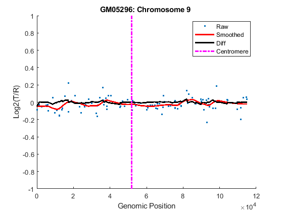
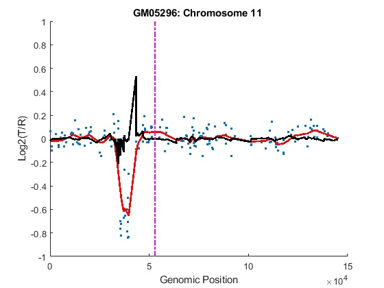
You can inspect the data by plotting the log2-based ratios, the smoothed ratios and the derivative of the smoothed ratios together. You can also display the centromere position of a chromosome in the data plots. The magenta vertical bar marks the centromere of the chromosome.
for iloop = 1:length(GM05296_Data)
    chr = GM05296_Data(iloop).Chromosome;
    chr_x = GM05296_Data(iloop).GenomicPosition;
    figure
    hold on
    plot(chr_x, GM05296_Data(iloop).Log2Ratio, '.');
    line(chr_x, GM05296_Data(iloop).SmoothedRatio,...
                'Color', 'r', 'LineWidth', 2);
    line(chr_x, GM05296_Data(iloop).DiffRatio,...
                'Color', 'k', 'LineWidth', 2);
    line([acen_pos(chr), acen_pos(chr)], [-1, 1],...
                'Color', 'm', 'LineWidth', 2, 'LineStyle', '-.');
    if iloop == 1
        legend('Raw','Smoothed','Diff', 'Centromere');
    end
    ylim([-1, 1])
    xlabel('Genomic Position')
    ylabel('Log2(T/R)')
    title(sprintf('GM05296: Chromosome %d ', chr))
    hold off
end

Detecting Change-Points
The derivatives of the smoothed ratio over a certain threshold usually indicate substantial changes with large peaks, and provide the estimate of the change-point indices. For this example you will select a threshold of 0.1.
thrd = 0.1;

for iloop = 1:length(GM05296_Data)
    idx = find(abs(GM05296_Data(iloop).DiffRatio) > thrd );
    N = numel(GM05296_Data(iloop).SmoothedRatio);
    GM05296_Data(iloop).SegIndex = [1;idx;N];

    % Number of possible segments found
    fprintf('%d segments initially found on Chromosome %d.\n',...
                 numel(GM05296_Data(iloop).SegIndex) - 1,...
                 GM05296_Data(iloop).Chromosome)
end
1 segments initially found on Chromosome 9.
4 segments initially found on Chromosome 10.
5 segments initially found on Chromosome 11.
Optimizing Change-Points by GM Clustering
Gaussian Mixture (GM) or Expectation-Maximization (EM) clustering can provide fine adjustments to the change-point indices [5]. The convergence to statistically optimal change-point indices can be facilitated by surrounding each index with equal-length set of adjacent indices. Thus each edge is associated with left and right distributions. The GM clustering learns the maximum-likelihood parameters of the two distributions. It then optimally adjusts the indices given the learned parameters.
You can set the length for the set of adjacent positions distributed around the change-point indices. For this example, you will select a length of 5. You can also inspect each change-point by plotting its GM clusters. In this example, you will plot the GM clusters for the Chromosome 10 data.
len = 5;
for iloop = 1:length(GM05296_Data)
    seg_num = numel(GM05296_Data(iloop).SegIndex) - 1;
    if seg_num > 1
        % Plot the data points in chromosome 10 data
        if GM05296_Data(iloop).Chromosome == 10
            figure
            hold on;
            plot(GM05296_Data(iloop).GenomicPosition,...
                 GM05296_Data(iloop).Log2Ratio, '.')
            ylim([-0.5, 1])
            xlabel('Genomic Position')
            ylabel('Log2(T/R)')
            title(sprintf('Chromosome %d - GM05296', ...
                GM05296_Data(iloop).Chromosome))
        end

        segidx = GM05296_Data(iloop).SegIndex;
        segidx_emadj = GM05296_Data(iloop).SegIndex;

        for jloop = 2:seg_num
            ileft = min(segidx(jloop) - len, segidx(jloop));
            iright = max(segidx(jloop) + len, segidx(jloop));
            gmx = GM05296_Data(iloop).GenomicPosition(ileft:iright);
            gmy = GM05296_Data(iloop).SmoothedRatio(ileft:iright);

            % Select initial guess for the cluster index for each point.
            gmpart = (gmy > (min(gmy) + range(gmy)/2)) + 1;

            % Create a Gaussian mixture model object
            gm = gmdistribution.fit(gmy, 2, 'start', gmpart);
            gmid = cluster(gm,gmy);

            segidx_emadj(jloop) = find(abs(diff(gmid))==1) + ileft;

          % Plot GM clusters for the change-points in chromosome 10 data
            if GM05296_Data(iloop).Chromosome == 10
                plot(gmx(gmid==1),gmy(gmid==1), 'g.',...
                     gmx(gmid==2), gmy(gmid==2), 'r.')
            end
        end

        % Remove repeat indices
        zeroidx = [diff(segidx_emadj) == 0; 0];
        GM05296_Data(iloop).SegIndex = segidx_emadj(~zeroidx);
    end

    % Number of possible segments found
    fprintf('%d segments found on Chromosome %d after GM clustering adjustment.\n',...
                 numel(GM05296_Data(iloop).SegIndex) - 1,...
                 GM05296_Data(iloop).Chromosome)
end
hold off;
1 segments found on Chromosome 9 after GM clustering adjustment.
3 segments found on Chromosome 10 after GM clustering adjustment.
5 segments found on Chromosome 11 after GM clustering adjustment.

Testing Change-Point Significance
Once you determine the optimal change-point indices, you also need to determine if each segment represents a statistically significant changes in DNA copy number. You will perform permutation t-tests to assess the significance of the segments identified. A segment includes all the data points from one change-point to the next change-point or the chromosome end. In this example, you will perform 10,000 permutations of the data points on two consecutive segments along the chromosome at the significance level of 0.01.
alpha = 0.01;
for iloop = 1:length(GM05296_Data)
    seg_num = numel(GM05296_Data(iloop).SegIndex) - 1;
    seg_index = GM05296_Data(iloop).SegIndex;
    if seg_num > 1
        ppvals = zeros(seg_num+1, 1);

        for sloop =  1:seg_num-1
            seg1idx = seg_index(sloop):seg_index(sloop+1)-1;

            if sloop== seg_num-1
                seg2idx = seg_index(sloop+1):(seg_index(sloop+2));
            else
                seg2idx = seg_index(sloop+1):(seg_index(sloop+2)-1);
            end

            seg1 = GM05296_Data(iloop).SmoothedRatio(seg1idx);
            seg2 = GM05296_Data(iloop).SmoothedRatio(seg2idx);

            n1 = numel(seg1);
            n2 = numel(seg2);
            N = n1+n2;
            segs = [seg1;seg2];

            % Compute observed t statistics
            t_obs = mean(seg1) - mean(seg2);

            % Permutation test
            iter = 10000;
            t_perm = zeros(iter,1);
            for i = 1:iter
                randseg = segs(randperm(N));
                t_perm(i) = abs(mean(randseg(1:n1))-mean(randseg(n1+1:N)));
            end
            ppvals(sloop+1) = sum(t_perm >= abs(t_obs))/iter;
        end

        sigidx = ppvals < alpha;
        GM05296_Data(iloop).SegIndex = seg_index(sigidx);
    end

    % Number segments after significance tests
    fprintf('%d segments found on Chromosome %d after significance tests.\n',...
       numel(GM05296_Data(iloop).SegIndex) - 1, GM05296_Data(iloop).Chromosome)
end
1 segments found on Chromosome 9 after significance tests.
3 segments found on Chromosome 10 after significance tests.
4 segments found on Chromosome 11 after significance tests.
Assessing Copy Number Alterations
Cytogenetic study indicates cell line GM05296 has a trisomy at 10q21-10q24 and a monosomy at 11p12-11p13 [3]. Plot the segment means of the three chromosomes over the original data with bold red lines, and add the chromosome ideograms to the plots using the chromosomeplot function. Note that the genomic positions in the Coriell cell line data set are in kilo base pairs. Therefore, you will need to convert cytoband data from bp to kilo bp when adding the ideograms to the plot.
for iloop = 1:length(GM05296_Data)
    figure;
    seg_num = numel(GM05296_Data(iloop).SegIndex) - 1;
    seg_mean = ones(seg_num,1);
    chr_num = GM05296_Data(iloop).Chromosome;
    for jloop = 2:seg_num+1
        idx = GM05296_Data(iloop).SegIndex(jloop-1):GM05296_Data(iloop).SegIndex(jloop);
        seg_mean(idx) = mean(GM05296_Data(iloop).Log2Ratio(idx));
        line(GM05296_Data(iloop).GenomicPosition(idx), seg_mean(idx),...
            'color', 'r', 'linewidth', 3);
    end
    line(GM05296_Data(iloop).GenomicPosition, GM05296_Data(iloop).Log2Ratio,...
        'linestyle', 'none', 'Marker', '.');
    line([acen_pos(chr_num), acen_pos(chr_num)], [-1, 1],...
        'linewidth', 2,...
        'color', 'm',...
        'linestyle', '-.');

    ylabel('Log2(T/R)')
    ax = gca;
    ax.Box = 'on';
    ylim([-1, 1])
    title(sprintf('Chromosome %d - GM05296', chr_num));
    chromosomeplot(hs_cytobands, chr_num, 'addtoplot', gca,  'unit', 2)

end
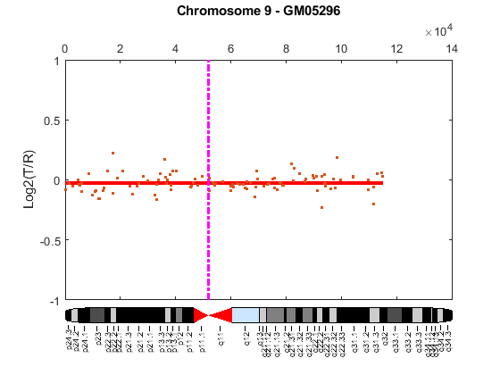
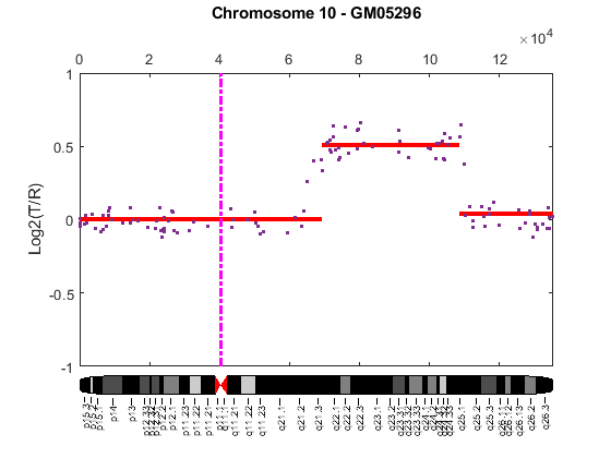
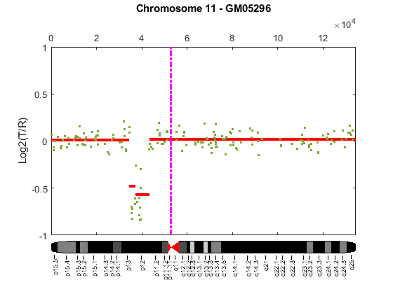
As shown in the plots, no copy number alterations were found on chromosome 9, there is copy number gain span from 10q21 to 10q24, and a copy number loss region from 11p12 to 11p13. The CNAs found match the known results in cell line GM05296 determined by cytogenetic analysis.
You can also display the CNAs of the GM05296 cell line align to the chromosome ideogram summary view using the chromosomeplot function. Determine the genomic positions for the CNAs on chromosomes 10 and 11.
chr10_idx = GM05296_Data(2).SegIndex(2):GM05296_Data(2).SegIndex(3)-1;
chr10_cna_start = GM05296_Data(2).GenomicPosition(chr10_idx(1))*1000;
chr10_cna_end   = GM05296_Data(2).GenomicPosition(chr10_idx(end))*1000;

chr11_idx = GM05296_Data(3).SegIndex(2):GM05296_Data(3).SegIndex(3)-1;
chr11_cna_start = GM05296_Data(3).GenomicPosition(chr11_idx(1))*1000;
chr11_cna_end = GM05296_Data(3).GenomicPosition(chr11_idx(end))*1000;
Create a structure containing the copy number alteration data from the GM05296 cell line data according to the input requirements of the chromosomeplot function.
cna_struct = struct('Chromosome', [10 11],...
                     'CNVType', [2 1],...
                     'Start', [chr10_cna_start, chr11_cna_start],...
                     'End',   [chr10_cna_end, chr11_cna_end])
cna_struct =

  struct with fields:

    Chromosome: [10 11]
       CNVType: [2 1]
         Start: [69209000 34420000]
           End: [105905000 35914000]
chromosomeplot(hs_cytobands, 'cnv', cna_struct, 'unit', 2)
title('Human Karyogram with Copy Number Alterations of GM05296')

This example shows how MATLAB and its toolboxes provide tools for the analysis and visualization of copy-number alterations in array-based CGH data.
References
[1] Redon, R., et al., "Global variation in copy number in the human genome", Nature, 444(7118):444-54, 2006.
[2] Pinkel, D., et al., "High resolution analysis of DNA copy number variations using comparative genomic hybridization to microarrays", Nature Genetics, 20(2):207-11, 1998.
[3] Snijders, A.M., et al., "Assembly of microarrays for genome-wide measurement of DNA copy number", Nature Genetics, 29(3):263-4, 2001.
[4] Human Genome NCBI Build 36.
[5] Myers, C.L., et al., "Accurate detection of aneuploidies in array CGH and gene expression microarray data", Bioinformatics, 20(18):3533-43, 2004.