Identifying Over-Represented Regulatory Motifs
This example illustrates a simple approach to searching for potential regulatory motifs in a set of co-expressed genomic sequences by identifying significantly over-represented ungapped words of fixed length. The discussion is based on the case study presented in Chapter 10 of "Introduction to Computational Genomics. A Case Studies Approach" [1].
Introduction
The circadian clock is the 24 hour cycle of the physiological processes that synchronize with the external day-night cycle. Most of the work on the circadian oscillator in plants has been carried out using the model plant Arabidopsis thaliana. In this organism, the regulation of a series of genes that need to be turned on or off at specific time of the day and night, is accomplished by small regulatory sequences found upstream the genes in question. One such regulatory motif, AAAATATCT, also known as the Evening Element (EE), has been identified in the promoter regions of circadian clock-regulated genes that show peak expression in the evening [2].
Loading Upstream Regions of Clock-Regulated Genes
We consider three sets of clock-regulated genes, clustered according to the time of the day when they are maximally expressed: set 1 corresponds to 1 KB-long upstream regions of genes whose expression peak in the morning (8am-4pm); set 2 corresponds to 1 KB-long upstream regions of genes whose expression peak in the evening (4pm-12pm); set 3 corresponds to 1 KB-long upstream regions of genes whose expression peak in the night (12pm-8am). Because we are interested in a regulatory motif in evening genes, set 2 represents our target set, while set 1 and set 3 are used as background. In each set, the sequences and their respective reverse complements are concatenated to each other, with individual sequences separated by a gap symbol (-).
load evemotifdemodata.mat;

% === concatenate both strands
s1 = [[set1.Sequence] seqrcomplement([set1.Sequence])];
s2 = [[set2.Sequence] seqrcomplement([set2.Sequence])];
s3 = [[set3.Sequence] seqrcomplement([set3.Sequence])];

% === compute length and number of sequences in each set
L1 = length(set1(1).Sequence);
L2 = length(set2(1).Sequence);
L3 = length(set3(1).Sequence);

N1 = numel(set1) * 2;
N2 = numel(set2) * 2;
N3 = numel(set3) * 2;

% === add separator between sequences
seq1 = seqinsertgaps(s1, 1:L1:(L1*N1)+N1, 1);
seq2 = seqinsertgaps(s2, 1:L2:(L2*N2)+N2, 1);
seq3 = seqinsertgaps(s3, 1:L3:(L3*N3)+N3, 1);
Identifying Over-Represented Words
To determine which candidate motif is over-represented in a given target set with respect to the background set, we identify all possible W-mers (words of length W) in both sets and compute their frequency. A word is considered over-represented if its frequency in the target set is significantly higher than the frequency in the background set. This difference is also called "margin".
type findOverrepresentedWords
function [nmersSorted, freqDiffSorted] = findOverrepresentedWords(seq, seq0, W)
% FINDOVERREPRESENTEDWORDS helper for evemotifdemo

% Copyright 2007 The MathWorks, Inc.

%=== find and count words of length W
nmers0 = nmercount(seq0, W);
nmers = nmercount(seq, W);

%=== compute frequency of words
f = [nmers{:,2}]/(length(seq) - W + 1);
f0 = [nmers0{:,2}]/(length(seq0) - W + 1);

%=== determine words common to both set
[nmersInt, i1, i2] = intersect(nmers(:,1),nmers0(:,1));
freqDiffInt = (f(i1) - f0(i2))';

%=== determine words specific to one set only
[nmersXOr, i3, i4] = setxor(nmers(:,1),nmers0(:,1));
c0 = nmers(i3,1);
d0 = nmers0(i4,1);
nmersXOr = [c0; d0];
freqDiffXOr = [f(i3) -f0(i4)]';

%=== define all words and their difference in frequency (margin)
nmersAll = [nmersInt; nmersXOr];
freqDiff = [freqDiffInt; freqDiffXOr];

%=== sort according to descending difference in frequency
[freqDiffSorted, freqDiffSortedIndex] = sort(freqDiff, 'descend');
nmersSorted = nmersAll(freqDiffSortedIndex);
The Evening Element Motif
If we consider all words of length W = 9 that appear more frequently in the target set (upstream region of genes highly expressed in the evening) with respect to the background set (upstream region of genes highly expressed in the morning and night), we notice that the most over-represented word is 'AAAATATCT', also known as the Evening Element (EE) motif.
W = 9;

[words, freqDiff] = findOverrepresentedWords(seq2, [seq1 seq3],W);
words(1:10)
freqDiff(1:10)
ans =

  10×1 cell array

    {'AAAATATCT'}
    {'AGATATTTT'}
    {'CTCTCTCTC'}
    {'GAGAGAGAG'}
    {'AGAGAGAGA'}
    {'TCTCTCTCT'}
    {'AAATATCTT'}
    {'AAGATATTT'}
    {'AAAAATATC'}
    {'GATATTTTT'}


ans =

   1.0e-03 *

    0.1439
    0.1439
    0.1140
    0.1140
    0.1074
    0.1074
    0.0713
    0.0713
    0.0695
    0.0695
Filtering out Repeats
Besides the EE motif, other words of length W = 9 appear to be over-represented in the target set. In particular, we notice the presence of repeats, i.e., words consisting of a single nucleotide or dimer repeated for the entire word length, such as 'CTCTCTCTC'. This phenomenon is quite common in genomic sequences and generally is associated with non-functional components. Because in this context the repeats are unlikely to be biologically significant, we filter them out.
% === determine repeats
wordsN = numel(words);
r = zeros(wordsN,1);

for i = 1:wordsN
    if (all(words{i}(1:2:end) == words{i}(1)) && ... % odd positions are the same
        all(words{i}(2:2:end) == words{i}(2)))       % even positions are the same
    r(i) = 1;
    end
end
r = logical(r);

% === filter out repeats
words = words(~r);
freqDiff = freqDiff(~r);

% === consider the top 10 motifs
motif = words(1:10)
margin = freqDiff(1:10)

EEMotif = motif{1}
EEMargin = margin(1)
motif =

  10×1 cell array

    {'AAAATATCT'}
    {'AGATATTTT'}
    {'AAATATCTT'}
    {'AAGATATTT'}
    {'AAAAATATC'}
    {'GATATTTTT'}
    {'AAATAAAAT'}
    {'ATTTTATTT'}
    {'TAAATAAAA'}
    {'TTTTATTTA'}


margin =

   1.0e-03 *

    0.1439
    0.1439
    0.0713
    0.0713
    0.0695
    0.0695
    0.0656
    0.0656
    0.0600
    0.0600


EEMotif =

    'AAAATATCT'


EEMargin =

   1.4393e-04
After removing the repeats, we observe that the EE motif ('AAAATATCT') and its reverse complement ('AGATATTTT') are at the top of the list. The other over-represented words are either simple variants of the EE motif, such as 'AAATATCTT', 'AAAAATATC', 'AAATATCTC', or their reverse complements, such as 'AAGATATTT', 'GATATTTTT', 'GAGATATTT'.
Assessing the Statistical Significance of Margins
Various techniques can be used to assess the statistical significance of the margin computed for the EE motif. For example, we can repeat the analysis using some control sequences and evaluate the resulting margins with respect to the EE margin. Genomic regions of Arabidopsis thaliana that are further away from the transcription start site are good candidates for this purpose. Alternatively, we could randomly split and shuffle the sequences under consideration and use these as controls. Another simple solution is to generate random sequences according to the nucleotide composition of the three original sets of sequences, as shown below.
% === find base composition of each set
bases1 = basecount(s1);
bases2 = basecount(s2);
bases3 = basecount(s3);

% === generate random sequences according to base composition
rs1  = randseq(length(s1),'fromstructure', bases1);
rs2  = randseq(length(s2),'fromstructure', bases2);
rs3  = randseq(length(s3),'fromstructure', bases3);

% === add separator between sequences
rseq1 = seqinsertgaps(rs1, 1:L1:(L1*N1)+N1, 1);
rseq2 = seqinsertgaps(rs2, 1:L2:(L2*N2)+N2, 1);
rseq3 = seqinsertgaps(rs3, 1:L3:(L3*N3)+N3, 1);

% === compute margins for control set
[words, freqDiff] = findOverrepresentedWords(rseq2, [rseq1 rseq3],W);
The variable ctrlMargin holds the estimated margins of the top motifs for each of the 100 control sequences generated as described above. The distribution of these margins can be approximated by the extreme value distribution. We use the function gevfit from the Statistics and Machine Learning Toolbox™ to estimate the parameters (shape, scale, and location) of the extreme value distribution and we overlay a scaled version of its probability density function, computed using gevpdf, with the histogram of the margins of the control sequences.
% === estimate parameters of distribution
nCtrl = length(ctrlMargin);
buckets = ceil(nCtrl/10);
parmhat = gevfit(ctrlMargin);
k = parmhat(1);     % shape parameter
sigma = parmhat(2); % scale parameter
mu = parmhat(3);    % location parameter

% === compute probability density function
x = linspace(min(ctrlMargin), max([ctrlMargin EEMargin]));
y = gevpdf(x, k, sigma, mu);

% === scale probability density function
[v, c] = hist(ctrlMargin,buckets);
binWidth = c(2) - c(1);
scaleFactor = nCtrl * binWidth;

% === overlay
figure()
hold on;
hist(ctrlMargin, buckets);
h = findobj(gca,'Type','patch');
h.FaceColor = [.9 .9 .9];
plot(x, scaleFactor * y, 'r');
stem(EEMargin, 1, 'b');
xlabel('Margin');
ylabel('Number of sequences');
legend('Ctrl Margins', 'EVD pdf', 'EE Margin');
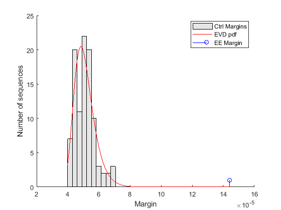
The control margins are the differences in frequency that we would expect to find when a word is over-represented by chance alone. The margin relative to the EE motif is clearly significantly larger than the control margins, and does not fit within the probability density curve of the random controls. Because the EE margin is larger than all 100 control margins, we can conclude that the over-representation of the EE motif in the target set is statistically significant and the p-value estimate is less than 0.01.
Selecting Motif Length
If we repeat the search for over-represented words of length W = 6...11, we observe that all the top motifs are either substrings (if W < 9) or superstrings (if W > 9) of the EE motif. Thus, how do we decide what is the correct length of this motif? We can expect that the optimal length maximizes the difference in frequency between the motif in the target set and the same motif in the background set. However, in order to compare the margin across different lengths, the margin must be normalized to account for the natural tendency of shorter words to occur more frequently. We perform this normalization by dividing each margin by the margin corresponding to the most over-represented word of identical length in a random set of sequences with a nucleotide composition similar to the target set. For convenience, the top over-represented words for length W = 6...11 and their margins are stored in the variables topMotif and topMargin. Similarly, the top over-represented words for length W = 6...11 and their margins in a random set are stored in the variables rTopMotif and rTopMargin.
% === top over-represented words, W = 6...11 in set 2 (evening)
topMotif
topMargin

% === top over-represented words, W = 6...11 in random set
rTopMotif
rTopMargin

% === compute score
score = topMargin ./ rTopMargin;
[bestScore, bestLength] =  max(score);

% === plot
figure()
plot(6:11, score(6:11));
xlabel('Motif length');
ylabel('Normalized margin');
title('Optimal motif length');
hold on
line([bestLength bestLength], [0 bestScore], 'LineStyle', '-.')
topMotif =

  11×1 cell array

    {0×0 double   }
    {0×0 double   }
    {0×0 double   }
    {0×0 double   }
    {0×0 double   }
    {'AATATC'     }
    {'AATATCT'    }
    {'AAATATCT'   }
    {'AAAATATCT'  }
    {'AAAAATATCT' }
    {'AAAAAATATCT'}


topMargin =

   1.0e-03 *

       NaN
       NaN
       NaN
       NaN
       NaN
    0.3007
    0.2607
    0.2074
    0.1439
    0.0648
    0.0424


rTopMotif =

  11×1 cell array

    {0×0 double   }
    {0×0 double   }
    {0×0 double   }
    {0×0 double   }
    {0×0 double   }
    {'ATTATA'     }
    {'TATAATA'    }
    {'TTATTAAA'   }
    {'GTTATTAAA'  }
    {'ATTATATATC' }
    {'ATGTTATTATT'}


rTopMargin =

   1.0e-03 *

       NaN
       NaN
       NaN
       NaN
       NaN
    0.5650
    0.2374
    0.0972
    0.0495
    0.0279
    0.0183
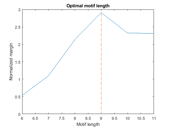
By plotting the normalized margin versus the motif length, we find that length W = 9 is the most informative in discriminating over-represented motifs in the target sequence (evening set) against the background set (morning and night sets).
Determining the Evening Element Motif Presence Among Clock-Regulated Genes
Although the EE Motif has been identified and experimentally validated as a regulatory motif for genes whose expression peaks in the evening hours, it is not shared by all evening genes, nor is it exclusive of these genes. We count the occurrences of the EE motif in the three sequence sets and determine what proportion of genes in each set contain the motif.
EECount = zeros(3,1);

% === determine positions where EE motif occurs
loc1 = strfind(seq1, EEMotif);
loc2 = strfind(seq2, EEMotif);
loc3 = strfind(seq3, EEMotif);

% === count occurrences
EECount(1) = length(loc1);
EECount(2) = length(loc2);
EECount(3) = length(loc3);

% === find proportions of genes with EE Motif
NumGenes = [N1; N2; N3] / 2;
EEProp = EECount ./ NumGenes;

% === plot
figure()
bar(EEProp, 0.5);
ylabel('Proportion of genes containing EE Motif');
xlabel('Gene set');
title('Presence of EE Motif');
ylim([0 1])
ax = gca;
ax.XTickLabel = {'morning', 'evening', 'night'};
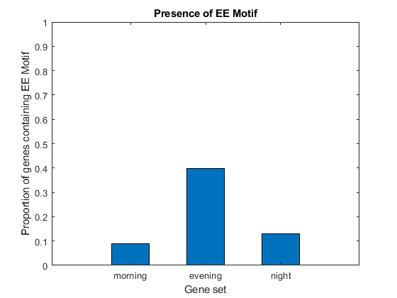
It appears as though about 9% of genes in set 1, 40% of genes in set 2, and 13% of genes in set 3 have the EE motif. Thus, not all genes in set 2 have the motif, but it is clearly enriched in this group.
Analyzing the Evening Element Motif Location
Unlike many other functional motifs, the EE motif does not appear to accumulate at specific gene locations in the set of sequences analyzed. After determining the location of each occurrence with respect to the transcription start site (TSS), we observe a relatively uniform distribution of occurrences across the upstream region of the genes considered, with the possible exception of the middle region (between 400 and 500 bases upstream of the TSS).
offset = rem(loc2, 1001);
figure();
hist(offset, 100);
xlabel('Offset in upstream region (TSS = 0)');
ylabel('Number of sequences');

References
[1] Cristianini, N. and Hahn, M.W., "Introduction to Computational Genomics: A Case Studies Approach", Cambridge University Press, 2007.
[2] Harmer, S.L., et al., "Orchestrated Transcription of Key Pathways in Arabidopsis by the Circadian Clock", Science, 290(5499):2110-3, 2000.