BER Performance of Different Equalizers

This example shows the BER performance of several types of equalizers in a static channel with a null in the passband. The example constructs and implements a linear equalizer object and a decision feedback equalizer (DFE) object. It also initializes and invokes a maximum likelihood sequence estimation (MLSE) equalizer. The MLSE equalizer is first invoked with perfect channel knowledge, then with a straightforward but imperfect channel estimation technique.

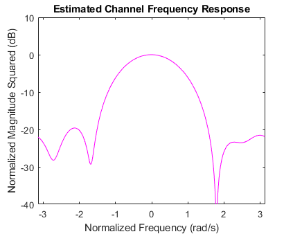
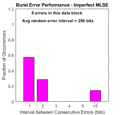
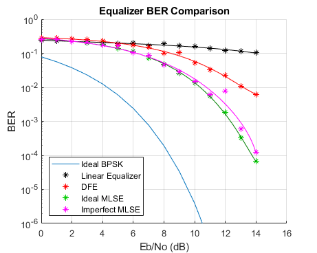
As the simulation progresses, it updates a BER plot for comparative analysis between the equalization methods. It also shows the signal spectra of the linearly equalized and DFE equalized signals. It also shows the relative burstiness of the errors, indicating that at low BERs, both the MLSE algorithm and the DFE algorithm suffer from error bursts. In particular, the DFE error performance is burstier with detected bits fed back than with correct bits fed back. Finally, during the "imperfect" MLSE portion of the simulation, it shows and dynamically updates the estimated channel response.

To experiment with this example, you can change such parameters as the channel impulse response, the number of equalizer tap weights, the recursive least squares (RLS) forgetting factor, the least mean square (LMS) step size, the MLSE traceback length, the error in estimated channel length, and the maximum number of errors collected at each Eb/No value.

Code Structure

This example relies on these helper scripts and functions to perform link simulations over a range of Eb/No values.

eqber_adaptive.m - a script that runs link simulations for linear and DFE equalizers

eqber_mlse.m - a script that runs link simulations for ideal and imperfect MLSE equalizers

eqber_siggen.m - a script that generates a binary phase shift keying (BPSK) signal with no pulse shaping, then processes it through the channel and adds noise

eqber_graphics.m - a function that generates and updates plots showing the performance of the linear, DFE, and MLSE equalizers.

The scripts eqber_adaptive and eqber_mlse illustrate how to use adaptive and MLSE equalizers across multiple blocks of data such that state information is retained between data blocks.

Signal and Channel Parameters

Set parameters related to the signal and channel. Use BPSK without any pulse shaping, and a 5-tap real-valued symmetric channel impulse response. (See section 10.2.3 of Digital Communications by J. Proakis, 4th Ed., for more details on the channel.) Set initial states of data and noise generators. Set the Eb/No range.

% System simulation parameters
Fs = 1;           % sampling frequency (notional)
nBits = 2048;     % number of BPSK symbols per vector
maxErrs = 200;    % target number of errors at each Eb/No
maxBits = 1e6;    % maximum number of symbols at each Eb/No

% Modulated signal parameters
M = 2;                     % order of modulation
Rs = Fs;                   % symbol rate
nSamp = Fs/Rs;             % samples per symbol
k = log2(M);               % Bits per symbol
Rb = Rs*k;                 % bit rate

% Channel parameters
chnl = [0.227 0.460 0.688 0.460 0.227]';  % channel impulse response
chnlLen = length(chnl);                   % channel length, in samples
EbNo = 0:14;                              % in dB
BER = zeros(size(EbNo));                  % initialize values

% Create BPSK modulator
bpskMod = comm.BPSKModulator;

% Specify a seed for the random number generators to ensure repeatability.
rng(12345)

Adaptive Equalizer Parameters

Set parameter values for the linear and DFE equalizers. Use a 31-tap linear equalizer, and a DFE with 15 feedforward and feedback taps. Use the recursive least squares (RLS) algorithm for the first block of data to ensure rapid tap convergence. Use the least mean square (LMS) algorithm thereafter to ensure rapid execution speed.

% Linear equalizer parameters
nWts = 31;               % number of weights
algType = 'RLS';         % RLS algorithm
forgetFactor = 0.999999; % parameter of RLS algorithm

% DFE parameters - use same update algorithms as linear equalizer
nFwdWts = 15;            % number of feedforward weights
nFbkWts = 15;            % number of feedback weights

MLSE Equalizer & Channel Estimation Parameters and Initial Visualization

Set the parameters of the MLSE equalizer. Use a traceback length of six times the length of the channel impulse response. Initialize the equalizer states. Set the equalization mode to "continuous", to enable seamless equalization over multiple blocks of data. Use a cyclic prefix in the channel estimation technique, and set the length of the prefix. Assume that the estimated length of the channel impulse response is one sample longer than the actual length.

% MLSE equalizer parameters
tbLen = 30;                        % MLSE equalizer traceback length
numStates = M^(chnlLen-1);         % number of trellis states
[mlseMetric,mlseStates,mlseInputs] = deal([]);
const = constellation(bpskMod);    % signal constellation
mlseType = 'ideal';                % perfect channel estimates at first
mlseMode = 'cont';                 % no MLSE resets

% Channel estimation parameters
chnlEst = chnl;         % perfect estimation initially
prefixLen = 2*chnlLen;  % cyclic prefix length
excessEst = 1;          % length of estimated channel impulse response
% beyond the true length

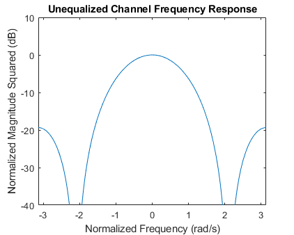
% Initialize the graphics for the simulation. Plot the unequalized channel
% frequency response, and the BER of an ideal BPSK system.
idealBER = berawgn(EbNo,'psk',M,'nondiff');

[hBER,hLegend,legendString,hLinSpec,hDfeSpec,hErrs,hText1,hText2, ...
    hFit,hEstPlot,hFig,hLinFig,hDfeFig] = eqber_graphics('init', ...
    chnl,EbNo,idealBER,nBits);

Construct RLS and LMS Linear and DFE Equalizer Objects

The RLS update algorithm is used to adapt the equalizer tap weights and reference tap is set to center tap.

linEq = comm.LinearEqualizer('Algorithm',algType, ...
    'ForgettingFactor',forgetFactor, ...
    'NumTaps',nWts, ...
    'Constellation',const, ...
    'ReferenceTap',round(nWts/2), ...
    'TrainingFlagInputPort',true);

dfeEq = comm.DecisionFeedbackEqualizer('Algorithm',algType, ...
    'ForgettingFactor',forgetFactor, ...
    'NumForwardTaps',nFwdWts, ...
    'NumFeedbackTaps',nFbkWts, ...
    'Constellation',const, ...
    'ReferenceTap',round(nFwdWts/2), ...
    'TrainingFlagInputPort',true);

Linear Equalizer

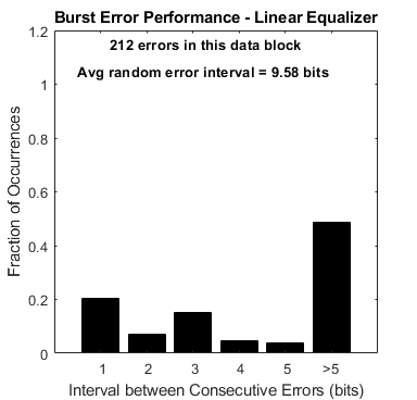
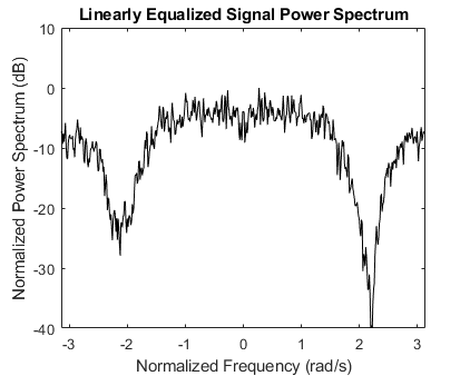
Run the linear equalizer, and plot the equalized signal spectrum, the BER, and the burst error performance for each data block. Note that as the Eb/No increases, the linearly equalized signal spectrum has a progressively deeper null. This highlights the fact that a linear equalizer must have many more taps to adequately equalize a channel with a deep null. Note also that the errors occur with small inter-error intervals, which is to be expected at such a high error rate.

See eqber_adaptive.m for a listing of the simulation code for the adaptive equalizers.

firstRun = true;  % flag to ensure known initial states for noise and data
eqType = 'linear';
eqber_adaptive;

Decision Feedback Equalizer

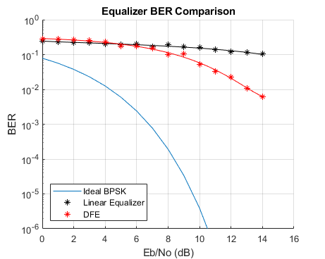
Run the DFE, and plot the equalized signal spectrum, the BER, and the burst error performance for each data block. Note that the DFE is much better able to mitigate the channel null than the linear equalizer, as shown in the spectral plot and the BER plot. The plotted BER points at a given Eb/No value are updated every data block, so they move up or down depending on the number of errors collected in that block. Note also that the DFE errors are somewhat bursty, due to the error propagation caused by feeding back detected bits instead of correct bits. The burst error plot shows that as the BER decreases, a significant number of errors occurs with an inter-error arrival of five bits or less. (If the DFE equalizer were run in training mode at all times, the errors would be far less bursty.)

For every data block, the plot also indicates the average inter-error interval if those errors were randomly occurring.

See eqber_adaptive.m for a listing of the simulation code for the adaptive equalizers.

close(hFig(ishghandle(hFig)));

eqType = 'dfe';
eqber_adaptive;

Ideal MLSE Equalizer, with Perfect Channel Knowledge

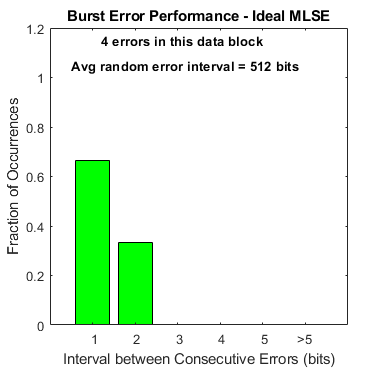
Run the MLSE equalizer with a perfect channel estimate, and plot the BER and the burst error performance for each data block. Note that the errors occur in an extremely bursty fashion. Observe, particularly at low BERs, that the overwhelming percentage of errors occur with an inter-error interval of one or two bits.

See eqber_mlse.m for a listing of the simulation code for the MLSE equalizers.

close(hLinFig(ishghandle(hLinFig)),hDfeFig(ishghandle(hDfeFig)));

eqType = 'mlse';
mlseType = 'ideal';
eqber_mlse;

MLSE Equalizer with an Imperfect Channel Estimate

Run the MLSE equalizer with an imperfect channel estimate, and plot the BER and the burst error performance for each data block. These results align fairly closely with the ideal MLSE results. (The channel estimation algorithm is highly dependent on the data, such that an FFT of a transmitted data block has no nulls.) Note how the estimated channel plots compare with the actual channel spectrum plot.

See eqber_mlse.m for a listing of the simulation code for the MLSE equalizers.

mlseType = 'imperfect';
eqber_mlse;