CSI Feedback with Transformer Autoencoder

Since R2024b

This example shows how to design and train a convolutional transformer deep neural network for channel state information (CSI) feedback by using a downlink clustered delay-line (CDL) channel model.

Introduction

Accurate CSI feedback at the base station (gNB) is essential to exploit the potential of massive multiple input multiple output (MIMO) systems in 5G networks. Deep learning (DL) CSI feedback methods can provide higher accuracy and lower overhead by learning the channel response features directly from the channel estimates instead of relying on prior assumptions. DL methods use deep autoencoder models that consist of jointly trained encoder and decoder networks. The user equipment (UE) uses the encoder network to compress the estimated channel parameters to a low dimensional codeword that is transmitted to the gNB. The gNB uses the decoder network to decompress the received codeword into the full channel parameters and compute the downlink transmission attributes, such as modulation scheme, code rate, and MIMO precoding.

CSI Feedback with Autoencoders example shows how to design, train, and test a convolutional neural network (CNN) autoencoder for CSI compression. Compared to CNN autoencoders, transformer networks can exploit long-term dependencies in data samples by using a self-attention mechanism. For CSI feedback, a transformer network can outperform a CNN in capturing the channel features across frequency subcarriers and transmit antennas.

In this example, you design, train, and test a convolutional transformer network for CSI compression [1]. Finally, you analyze the accuracy and complexity of the network for different compression rates.

Prepare Data Set

For this example, you use preprocessed data set of downlink CDL channel perfect estimates. The data set is generated using the helperCSIFormerGenerateDataset script with the following parameters:

• Tx Antennas: 32

• Rx Antennas: 2

• Delay Profile: CDL-B

• RMS delay spread: 100 ns

• Max delay after truncation: 32

• Max Doppler: 2 Hz

• Resource blocks: 48

• Subcarrier spacing: 30 KHz

By default, this example downloads the dataset from https://ssd.mathworks.com/supportfiles/spc/coexecutionPrecoding/processedData.zip. If you do not have an Internet connection, you can download the files manually on a computer that is connected to the Internet, and then unzip and save them to the example directory. To generate and preprocess a data set with different channel parameters, use the helperCSIFormerGenerateDataset script to set the new channel parameters and set datasetSource to generateDataset.

datasetSource = "downloadDataset";

if strcmp(datasetSource,"downloadDataset")
    helperDownloadFiles();
else
    helperCSIFormerGenerateDataset;%#ok
end

Starting download data set.
Downloading data set. Extracting files.
Extraction complete.

In the downloaded data set, the training and validation files are MAT files with the prefixes CDLChannelEst_train and CDLChannelEst_val, respectively. Read the data using a signalDatastore object and load it into memory using the readall function.

trainSds = signalDatastore(fullfile(pwd,"processedData","CDLChannelEst_train*"));
HTrainRealCell = readall(trainSds);
HTrainReal = cat(1,HTrainRealCell{:});
HTrainReal = permute(HTrainReal,[2,3,4,1]);
numTrainSamples = size(HTrainReal, 4)

numTrainSamples = 
10008

valSds = signalDatastore(fullfile(pwd,"processedData","CDLChannelEst_val*"));
HValRealCell = readall(valSds);
HValReal = cat(1,HValRealCell{:});
HValReal = permute(HValReal,[2,3,4,1]);
numValSamples = size(HValReal, 4)

numValSamples = 
3000

Design Convolutional Transformer Network

This section implements the building blocks of a convolutional transformer autoencoder network based on [1], focusing on the encoder network. The decoder network uses the same blocks of layers. The main building blocks of layers in the network are:

• Flattened patch block

• Linear patch embedding layer

• Position patch embedding layer

• Window transformer block

• Unpatched convolution block

Use the imageInputLayer (Deep Learning Toolbox) function with input size [maxDelay numTx numChannels] to pass the input full channel estimates to the convolution2dLayer (Deep Learning Toolbox) function with filter size [5 5] and 16 output filters for an embedding size of 16. maxDelay is the truncated input size in the delay domain after preprocessing, numTx is the number of transmit antennas, and numChannels is the number inputs changes for the real and imaginary parts of the channel estimates. For details on the preprocessing steps of channel estimates for feedback compression, see CSI Feedback with Autoencoders example.

inputSize = size(HTrainReal(:,:,:,1))

inputSize = 1×3

    32    32     2

encodedSize is the number of elements in the compressed codeword at the encoder output. Set encodedSize to 64 and calculate the encoder compression rate.

encodedSize = 64;
compressionFactor = prod(inputSize)/encodedSize;
disp("Compression rate of the autoencoder is " + num2str(compressionFactor) +":1")

Compression rate of the autoencoder is 32:1

embeddingSize = 16;
encInputConvBlock = [imageInputLayer(inputSize, Name="enc_input")
    convolution2dLayer([5 5],embeddingSize,Padding=[2 2 2 2],Name="enc_conv2D")];

Use the convolution2dLayer function with filter size [2 2], stride [2 2], and 16 output filters to create patches of size [2 2] and embedding dimension of size 16. Flatten the first two dimensions of the output patches using a functionLayer (Deep Learning Toolbox) function with a reshape operation.

numPatches = inputSize(1)*inputSize(2)/(2*2);
flattenedPatchBlock = [convolution2dLayer([2 2], embeddingSize, Stride=[2 2], Name="enc_patches")
    functionLayer(@(X) dlarray(reshape(X,numPatches,embeddingSize,[]), 'SCB'), ...
    Formattable=true, Name="enc_flatten")
    ];

Use the helperCSIFormerLinearProjectionLayer function to create a linear projection layer. Given the flattened patches $$x\in R^{N*D}$$, the output of the linear projection layer, $$Y\in R^{N*D}$$, is given by$$Y=XE,$$ where $$E\in R^{D*D}$$ is a learnable linear projection matrix. $$N$$ is the number of patches and $$D$$ is the embedding dimension.

linearProjLayer = helperCSIFormerLinearProjectionLayer(embeddingSize, Name="enc_linearProject");

Create a deep learning network by using the dlnetwork (Deep Learning Toolbox) function and include the input convolution block, flattened patch block and linear projection layer.

net = dlnetwork([encInputConvBlock
    flattenedPatchBlock
    linearProjLayer]);

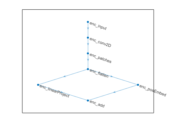
Use the positionEmbeddingLayer (Deep Learning Toolbox) function to embed the positions of the flattened patches over the spatial dimension and add the position embedding to the linear projection layer output.

posEmbedLayer =  positionEmbeddingLayer(embeddingSize,numPatches, ...
    PositionDimension="spatial", Name="enc_posEmbed");

net = addLayers(net, posEmbedLayer);
net = connectLayers(net,"enc_flatten","enc_posEmbed");
addLayer1 = additionLayer(2, Name="enc_add");
net = addLayers(net, addLayer1);
net = connectLayers(net,"enc_linearProject","enc_add/in1");
net = connectLayers(net,"enc_posEmbed","enc_add/in2");
plot(net)

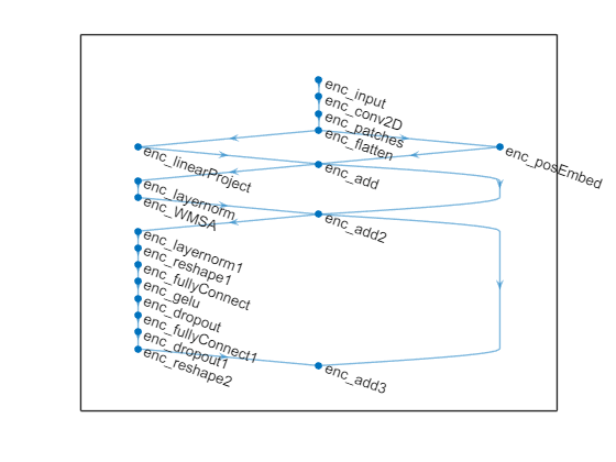
Use the layerNormalizationLayer (Deep Learning Toolbox) function followed by a Window-based multi-headed self-attention (W-MSA) layers block with a residual connection between the previous block input and the output of the self-attention layer. The W-MSA layers block is followed by a machine learning perceptron (MLP) block that consists of fully connected layers with Gaussian error linear unit (GELU) activations and dropout layers. Set the window size of the W-MSA block to 8.

windowSize = 8;
net = helperAddWMSALayersBlock(net,"enc_add",'enc_',windowSize);
plot(net)

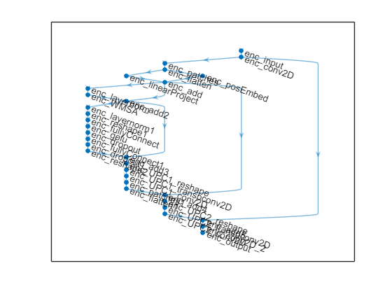
Create the unpatched convolution (UPC) block, that is, a full sized convolution, using a reshape function layer, transposed 2D convolutional layer, and a 2D convolutional layer. The UPC layers block is followed by a flatten patch layers block and a second UPC layers block.

net = helperAddUnpatched2DConvLayersBlock(net,"enc_add3",'enc_UPC1_');
net = helperAddFlattenPatchLayersBlock(net,"enc_UPC1_conv2D",'enc_',numPatches,embeddingSize);

addLayer4 = additionLayer(2, Name="enc_add4");
net = addLayers(net, addLayer4);
net = connectLayers(net,"enc_add","enc_add4/in1");
net = connectLayers(net,"enc_flatten1","enc_add4/in2");

net = helperAddUnpatched2DConvLayersBlock(net,"enc_add4",'enc_UPC2_');

addLayer5 = additionLayer(2, Name="enc_add5");
net = addLayers(net, addLayer5);
net = connectLayers(net,"enc_conv2D","enc_add5/in1");
net = connectLayers(net,"enc_UPC2_conv2D","enc_add5/in2");

Finally, use the convolution2dLayer function followed by the fullyConnectedLayer (Deep Learning Toolbox) function with output size encodedSize to output the encoded codeword.

encOutputConvBlock = [convolution2dLayer([3 3], 2, Padding=[1 1], Name="enc_conv2D_2")
    fullyConnectedLayer(encodedSize, Name="enc_output")];
net = addLayers(net, encOutputConvBlock);
CSIFormerEnc = connectLayers(net,"enc_add5","enc_conv2D_2");
plot(CSIFormerEnc)

The decoder network uses the same architecture as the encoder. Use the helperCSIFormerCreateNetwork function to create the complete network.

CSIFormerNet = helperCSIFormerCreateNetwork(inputSize,encodedSize, ...
    embeddingSize,numPatches,windowSize);
netAnalysis = analyzeNetwork(CSIFormerNet);
fprintf('Total number of learnables is  %.3f M.',netAnalysis.TotalLearnables/1e6);

Total number of learnables is  0.324 M.

Train Network

A warm-up period in the beginning of training a transformer network helps the network converge to a better local solution. To use a custom sequence of training schedules, create a cell array of warmupLearnRate (Deep Learning Toolbox) object followed by the built-in polynomial learning rate schedule. For information about learning rate schedules, see the trainingOptions (Deep Learning Toolbox)function. Use the local function helperNMSELossdB as a metric to plot the normalized mean square error (NMSE) in dB between the network inputs and outputs during training.

schedule = {warmupLearnRate( ...
    NumSteps=30, ...
    FrequencyUnit="epoch"), ...
    "polynomial"
    };

trainingMetric = @(x,t) helperNMSELossdB(x,t);

Set the maximum number of epochs to 1000, the batch size to 500, and the initial learning rate to 8e-4.

epochs = 1000;
batchSize = 500;
initLearnRate = 8e-4;

By default, the example loads a pretrained network with the selected encoded codeword size. To train the network from scratch, set the trainNow flag to true. Adjust the saveNetwork flag to save the trained network.

trainNow = false;
saveNetwork = false;

options = trainingOptions("adam", ...
    InitialLearnRate=initLearnRate, ...
    LearnRateSchedule=schedule, ...
    MaxEpochs=epochs, ...
    MiniBatchSize=batchSize, ...
    Shuffle="every-epoch", ...
    Verbose=false, ...
    VerboseFrequency=100, ...
    ValidationData={HValReal,HValReal}, ...
    ValidationFrequency=200, ...
    OutputNetwork="best-validation-loss", ...
    Metrics=trainingMetric, ...
    Plots="training-progress");

if trainNow
    [trainedNet, trainInfo] = trainnet(HTrainReal,HTrainReal,CSIFormerNet,@(X,T) mse(X,T),options);%#ok

    if saveNetwork
        save("CSIFormerTrainedNetwork_" ...
            + string(datetime("now","Format","dd_MM_HH_mm")), 'trainedNet')
    end

else
    trainedNetName = "trainedNetEnc" + num2str(compressionFactor);
    load("CSIFormerTrainedNets.mat",trainedNetName)
end

Test Trained Network

The downloaded data set contains test samples in MAT files with the prefix CDLChannelEst_test. Read and load the test data into memory.

testSds = signalDatastore(fullfile(pwd,"processedData","CDLChannelEst_test*"));
HTestRealCell = readall(testSds);
HTestReal = cat(1,HTestRealCell{:});
HTestReal = permute(HTestReal,[2,3,4,1]);
numTestSamples = size(HTestReal,4)

numTestSamples = 
2004

Test the accuracy of the trained network over the test data set using the testnet (Deep Learning Toolbox) function. Create a cell array of metric functions to compute the average value of each metric over the test samples. The NMSE in dB and the cosine similarity coefficient are typical metrics to evaluate the CSI feedback and recovery performance. Use the local functions helperMeanNMSELossdB and helperMeanCosineSimilarity as metrics for the testnet function.

testMetrics = {@(x,t) helperNMSELossdB(x,t),@(x,t) helperMeanCosineSimilarity(x,t)};

if ~trainNow
    switch compressionFactor
        case 16
            trainedNet = trainedNetEnc16;
        case 32
            trainedNet = trainedNetEnc32;
        case 64
            trainedNet = trainedNetEnc64;
    end    
end

testResults = testnet(trainedNet,HTestReal,HTestReal,testMetrics);
trainedNetInfo = analyzeNetwork(trainedNet,Plots="none");
totalLearnablesM = trainedNetInfo.TotalLearnables'/1e6;

resultsTable = table(categorical(num2str(compressionFactor) +":1"), ...
    testResults(1,1), testResults(1,2), totalLearnablesM, ...
    RowNames="trainedNet", ...
    VariableNames=[ "Compression Rate", "NMSE (dB)", "Cosine Similarity", "# Learnables (M)"]);

disp(resultsTable)

                  Compression Rate    NMSE (dB)    Cosine Similarity    # Learnables (M)
                  ________________    _________    _________________    ________________

    trainedNet          32:1           -39.823          0.99995             0.32416     

Compare Compression Rates Accuracy

This section compares the average NMSE, cosine similarity coefficient, and total number of parameters for the pretrained networks corresponding to compression rates 16:1, 32:1, and 64:1. For compression rate 16:1, the encoder maps a channel response estimate of size [32 32 2] to a vector of size [128 1] resulting in the highest cosine similarity coefficient value and the lowest NMSE value. However, mapping the channel response to a 128-dimensional space requires the highest number of learnables for the encoder and decoder networks. Since the network can only retain a smaller amount of information, the cosine similarity coefficient decreases and the NMSE increases as the compression factor increases. Similarly, mapping the channel response to a smaller dimensional space requires lower number of learnables for the encoder and decoder networks.

load CSIFormerComparisonResults

comparisonTable = table(categorical({'16:1'; '32:1'; '64:1'}), ...
    compareNMSE, compareCosineSim, compareLearnables, ...
    RowNames=["CSIFormer16", "CSIFormer32", "CSIFormer64"], ...
    VariableNames=[ "Compression Rate", "NMSE (dB)", "Cosine Similarity", "# Learnables (M)"]);

disp(comparisonTable)

                   Compression Rate    NMSE (dB)    Cosine Similarity    # Learnables (M)
                   ________________    _________    _________________    ________________

    CSIFormer16          16:1           -47.052          0.99999             0.58637     
    CSIFormer32          32:1           -39.823          0.99995             0.32416     
    CSIFormer64          64:1           -34.885          0.99985             0.19306     

Summary

In this example, you learned how to implement, train and test a convolutional transformer autoencoder network for CSI feedback compression. Comparison results shows the loss in accuracy and reduction in the network for higher feedback compression rates.

Helper Functions

helperCSIFormerGenerateDataset

helperCSIFormerCreateNetwork

helperCSIFormerLinearProjectionLayer

helperCSIFormerWindowSelfAttentionLayer

Local Functions

Custom Layer Blocks

function net = helperAddWMSALayersBlock(net,previousLayer,layersPrefix,windowSize)
%HELPERADDWMSALAYERSBLOCK Add a window-based multi-headed self-attention (W-MSA) layers block

W_MSABlock = [layerNormalizationLayer(Name=[layersPrefix 'layernorm'])
    helperCSIFormerWindowSelfAttentionLayer(1, 16, 16, windowSize, Name=[layersPrefix 'WMSA'])
    ];
net = addLayers(net, W_MSABlock);
net = connectLayers(net,previousLayer,[layersPrefix 'layernorm']);
addLayer2 = additionLayer(2, Name=[layersPrefix 'add2']);
net = addLayers(net, addLayer2);
net = connectLayers(net,previousLayer,[layersPrefix 'add2/in1']);
net = connectLayers(net,[layersPrefix 'WMSA'],[layersPrefix 'add2/in2']);

MLPBlock = [layerNormalizationLayer(Name=[layersPrefix 'layernorm1'])
    functionLayer(@(X) dlarray(X, 'TCB'), Formattable=true, Name=[layersPrefix 'reshape1'])
    fullyConnectedLayer(256, Name=[layersPrefix 'fullyConnect'])
    geluLayer(Name=[layersPrefix 'gelu'])
    dropoutLayer(0.1, Name=[layersPrefix 'dropout'])
    fullyConnectedLayer(16, Name=[layersPrefix 'fullyConnect1'])
    dropoutLayer(0.1, Name=[layersPrefix 'dropout1'])
    functionLayer(@(X) dlarray(X, 'CBS'), Formattable=true, Name=[layersPrefix 'reshape2'])];

net = addLayers(net, MLPBlock);
net = connectLayers(net,[layersPrefix 'add2'],[layersPrefix 'layernorm1']);

addLayer3 = additionLayer(2, Name=[layersPrefix 'add3']);
net = addLayers(net, addLayer3);
net = connectLayers(net,[layersPrefix 'add2'],[layersPrefix 'add3/in1']);
net = connectLayers(net,[layersPrefix 'reshape2'],[layersPrefix 'add3/in2']);

end

function net = helperAddUnpatched2DConvLayersBlock(net,previousLayer,layersPrefix)
%HELPERADDUNPATCHED2DCONVBLOCK Add an unpatched 2D convolution layers block

UPCBlock = [functionLayer(@(X) dlarray(reshape(stripdims(X), 16, 16, 16, []), "SSCB"), Formattable=true, Name=[layersPrefix 'reshape'])
    transposedConv2dLayer([4 4], 16, Stride=2, Cropping=1, Name=[layersPrefix 'transpconv2D'])
    convolution2dLayer([3 3], 16, Padding=[1 1], Name=[layersPrefix 'conv2D'])];

net = addLayers(net, UPCBlock);
net = connectLayers(net,previousLayer,[layersPrefix 'reshape']);
end

function net = helperAddFlattenPatchLayersBlock(net,previousLayer,layersPrefix,numPatches,embeddingSize)
%HELPERADDFLATTENEDPATCHBLOCK Add a flatten patch layers block

flattenPatchBlock1 = [convolution2dLayer([2 2],embeddingSize, ...
    Stride=[2 2],Name=[layersPrefix 'patches1'])
    functionLayer(@(X) dlarray(reshape(X,numPatches,embeddingSize,[]), 'SCB'), ...
    Formattable=true, Name=[layersPrefix ,'flatten1'])];
net = addLayers(net, flattenPatchBlock1);
net = connectLayers(net,previousLayer,"enc_patches1");
end

Custom Metrics

function loss = helperNMSELossdB(x,xHat)
%HELPERNMSELOSSDB NMSE loss in dB

% Combine real and imaginary parts
in = complex(x(:,:,1,:),x(:,:,2,:));
out = complex(xHat(:,:,1,:),xHat(:,:,2,:));
nmsePerObservation = helperNMSE(in,out);
loss = mean(nmsePerObservation);
end

function meanRho = helperMeanCosineSimilarity(x,xHat)
%HELPERMEANCOSINESIMILARITY Cosine similarity coefficient

% Combine real and imaginary parts
in = squeeze(complex(x(:,:,1,:),x(:,:,2,:)));
out = squeeze(complex(xHat(:,:,1,:),xHat(:,:,2,:)));

% Compute the average cosine similarity over subcarriers
rhoPerSample = helperComplexCosineSimilarity(in,out);
meanRho = mean(abs(rhoPerSample));
end

Data Set Download

function helperDownloadFiles()
% Download CDL Channel model data set
targetDir = 'coexecutionPrecoding/processedData';
name  = 'data set';

dstFolder = pwd;
folderName = 'processedData';
    
if exist(folderName,"dir")
    fprintf([folderName,' folder exists. Skip download.\n\n']);
else
    fprintf(['Starting download ',name,'.\n'])
    fileFullPath = matlab.internal.examples.downloadSupportFile('spc/', ...
        [targetDir,'.zip']);
    fprintf(['Downloading ',name,'. Extracting files.\n'])
    unzip(fileFullPath,dstFolder);
    fprintf('Extraction complete.\n\n')
end
end

References

[1] Bi, X., Li, S., Yu, C., and Zhang, Y., 2022. A novel approach using convolutional transformer for massive MIMO CSI feedback. IEEE Wireless Communications Letters, 11(5), pp.1017–1021.