lqgtrack

Form Linear-Quadratic-Gaussian (LQG) servo controller

Syntax

C = lqgtrack(kest,k)
C = lqgtrack(kest,k,'2dof')
C = lqgtrack(kest,k,'1dof')
C = lqgtrack(kest,k,...CONTROLS)


Description

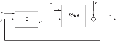
lqgtrack forms a Linear-Quadratic-Gaussian (LQG) servo controller with integral action for the loop shown in the following figure. This compensator ensures that the output y tracks the reference command r and rejects process disturbances w and measurement noise v. lqgtrack assumes that r and y have the same length.

Note

Always use positive feedback to connect the LQG servo controller C to the plant output y.

C = lqgtrack(kest,k) forms a two-degree-of-freedom LQG servo controller C by connecting the Kalman estimator kest and the state-feedback gain k, as shown in the following figure. C has inputs $$[r;y]$$ and generates the command $$u=-K\left[\widehat{x};x_i\right]$$, where$$\widehat{x}$$ is the Kalman estimate of the plant state, and x_i is the integrator output.

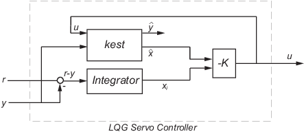
The size of the gain matrix k determines the length of x_i. x_i, y, and r all have the same length.

The two-degree-of-freedom LQG servo controller state-space equations are

$$\begin{array}{l}\left[\begin{array}{c}\dot{\widehat{x}}\\ {\dot{x}}_i\end{array}\right]=\left[\begin{array}{cc}A-B{K}_x-LC+LD{K}_x& -B{K}_i+LD{K}_i\\ 0& 0\end{array}\right]\left[\begin{array}{c}\widehat{x}\\ x_i\end{array}\right]+\left[\begin{array}{cc}0& L\\ I& -I\end{array}\right]\left[\begin{array}{c}r\\ y\end{array}\right]\\ u=\left[\begin{array}{cc}-K_x& -K_i\end{array}\right]\left[\begin{array}{c}\widehat{x}\\ x_i\end{array}\right]\end{array}$$

Note

The syntax C = lqgtrack(kest,k,'2dof') is equivalent to C = lqgtrack(kest,k).

C = lqgtrack(kest,k,'1dof') forms a one-degree-of-freedom LQG servo controller C that takes the tracking error e = r – y as input instead of [r ; y], as shown in the following figure.

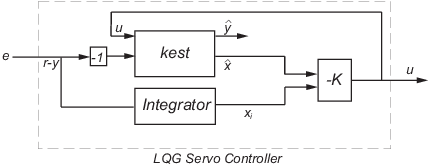
The one-degree-of-freedom LQG servo controller state-space equations are

$$\begin{array}{l}\left[\begin{array}{c}\dot{\widehat{x}}\\ {\dot{x}}_i\end{array}\right]=\left[\begin{array}{cc}A-B{K}_x-LC+LD{K}_x& -B{K}_i+LD{K}_i\\ 0& 0\end{array}\right]\left[\begin{array}{c}\widehat{x}\\ x_i\end{array}\right]+\left[\begin{array}{c}-L\\ I\end{array}\right]e\\ u=\left[\begin{array}{cc}-K_x& -K_i\end{array}\right]\left[\begin{array}{c}\widehat{x}\\ x_i\end{array}\right]\end{array}$$

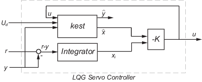
C = lqgtrack(kest,k,...CONTROLS) forms an LQG servo controller C when the Kalman estimator kest has access to additional known (deterministic) commands U_d of the plant. In the index vector CONTROLS, specify which inputs of kest are the control channels u. The resulting compensator C has inputs

• [U_d ; r ; y] in the two-degree-of-freedom case

• [U_d ; e] in the one-degree-of-freedom case

The corresponding compensator structure for the two-degree-of-freedom cases appears in the following figure.

Examples

See the example Design an LQG Servo Controller.

Tips

You can use lqgtrack for both continuous- and discrete-time systems.

In discrete-time systems, integrators are based on forward Euler (see lqi for details). The state estimate $$\widehat{x}$$ is either x[n|n] or x[n|n–1], depending on the type of estimator (see kalman for details).

For a discrete-time plant with equations:

$$\begin{array}{c}x\left[n+1\right]=Ax\left[n\right]+Bu\left[n\right]+Gw\left[n\right]\\ y\left[n\right]=Cx\left[n\right]+Du\left[n\right]+Hw\left[n\right]+v\left[n\right]\left\{\text{Measurements}\right\}\end{array}$$

connecting the "current" Kalman estimator to the LQR gain is optimal only when $$E\left(w\left[n\right]v{\left[n\right]}^{\prime }\right)=0$$ and y[n] does not depend on w[n] (H = 0). If these conditions are not satisfied, compute the optimal LQG controller using lqg.

Version History

Introduced in R2008b