Creating Discrete-Time Models

This example shows how to create discrete-time linear models using the tf, zpk, ss, and frd commands.

Specifying Discrete-Time Models

Control System Toolbox™ lets you create both continuous-time and discrete-time models. The syntax for creating discrete-time models is similar to that for continuous-time models, except that you must also provide a sample time (sampling interval in seconds).

For example, to specify the discrete-time transfer function:

$H (z) = \frac{z - 1}{z^{2} - 1.85 z + 0.9}$

with sampling period Ts = 0.1 s, type:

num = [ 1  -1 ];
den = [ 1  -1.85  0.9 ];
H = tf(num,den,0.1)

H =
 
        z - 1
  ------------------
  z^2 - 1.85 z + 0.9
 
Sample time: 0.1 seconds
Discrete-time transfer function.

or equivalently:

z = tf('z',0.1);
H = (z - 1) / (z^2 - 1.85*z + 0.9);

Similarly, to specify the discrete-time state-space model:

$x [k + 1] = 0.5 x [k] + u [k]$

$y [k] = 0.2 x [k] .$

with sampling period Ts = 0.1 s, type:

sys = ss(.5,1,.2,0,0.1);

Recognizing Discrete-Time Systems

There are several ways to determine if your LTI model is discrete:

The display shows a nonzero sample time value
sys.Ts or get(sys,'Ts') return a nonzero sample time value.
isdt(sys) returns true.

For example, for the transfer function H specified above,

H.Ts

ans = 
0.1000

isdt(H)

ans = logical
   1

You can also spot discrete-time systems by looking for the following traits:

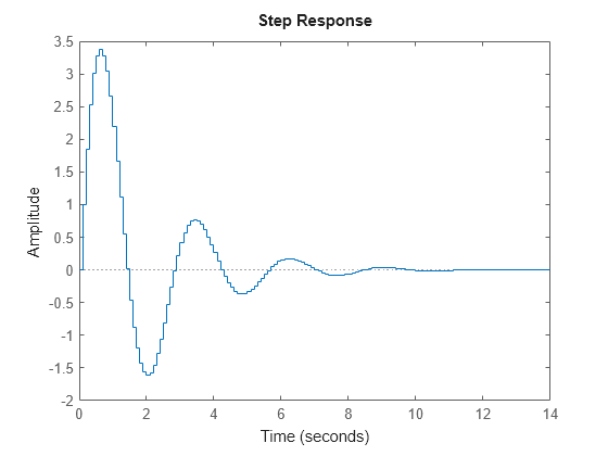
Time response plots - Response curve has a staircase look owing to its sampled-data nature
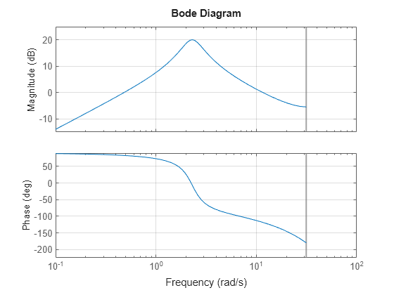
Bode plots - There is a vertical bar marking the Nyquist frequency (pi divided by the sample time).

The following plots show these characteristic traits:

step(H)

MATLAB figure

bode(H), grid

MATLAB figure