Tune 2-DOF PID Controller (Command Line)
This example shows how to design a two-degree-of-freedom (2-DOF) PID controller at the command line. The example also compares the 2-DOF controller performance to the performance achieved with a 1-DOF PID controller.
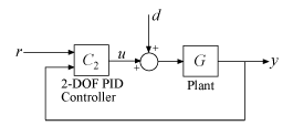
2-DOF PID controllers include setpoint weighting on the proportional and derivative terms. Compared to a 1-DOF PID controller, a 2-DOF PID controller can achieve better disturbance rejection without significant increase of overshoot in setpoint tracking. A typical control architecture using a 2-DOF PID controller is shown in the following diagram.
For this example, design a 2-DOF controller for the plant given by:

Suppose that your target bandwidth for the system is 1.5 rad/s.
wc = 1.5;
G = tf(1,[1 0.5 0.1]);
C2 = pidtune(G,'PID2',wc)
C2 =

                       1
  u = Kp (b*r-y) + Ki --- (r-y) + Kd*s (c*r-y)
                       s

  with Kp = 1.26, Ki = 0.255, Kd = 1.38, b = 0.665, c = 0

Continuous-time 2-DOF PID controller in parallel form.
Using the type 'PID2' causes pidtune to generate a 2-DOF controller, represented as a pid2 object. The display confirms this result. pidtune tunes all controller coefficients, including the setpoint weights b and c, to balance performance and robustness.
To compute the closed-loop response, note that a 2-DOF PID controller is a 2-input, 1-output dynamic system. You can resolve the controller into two channels, one for the reference signal and one for the feedback signal, as shown in the diagram. (See Continuous-Time 2-DOF PID Controller Representations for more information.)
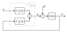
Decompose the controller into the components Cr and Cy, and use them to compute the closed-loop response from r to y.
C2tf = tf(C2);
Cr = C2tf(1);
Cy = C2tf(2);
T2 = Cr*feedback(G,Cy,+1);
To examine the disturbance-rejection performance, compute the transfer function from d to y.
S2 = feedback(G,Cy,+1);
For comparison, design a 1-DOF PID controller with the same bandwidth and compute the corresponding transfer functions. Then compare the step responses.
C1 = pidtune(G,'PID',wc);
T1 = feedback(G*C1,1);
S1 = feedback(G,C1);

subplot(2,1,1)
stepplot(T1,T2)
title('Reference Tracking')
subplot(2,1,2)
stepplot(S1,S2)
title('Disturbance Rejection')
legend('1-DOF','2-DOF')
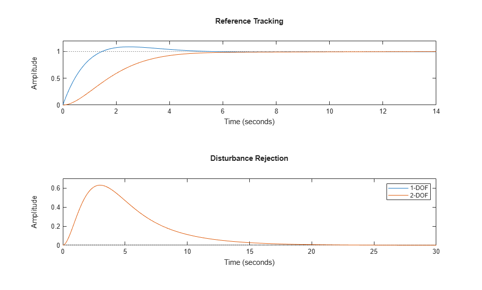
The plots show that adding the second degree of freedom eliminates the overshoot in the reference-tracking response without any cost to disturbance rejection. You can improve disturbance rejection too using the DesignFocus option. This option causes pidtune to favor disturbance rejection over setpoint tracking.
opt = pidtuneOptions('DesignFocus','disturbance-rejection');
C2dr = pidtune(G,'PID2',wc,opt)
C2dr =

                       1
  u = Kp (b*r-y) + Ki --- (r-y) + Kd*s (c*r-y)
                       s

  with Kp = 1.72, Ki = 0.593, Kd = 1.25, b = 0.029, c = 0

Continuous-time 2-DOF PID controller in parallel form.
With the default balanced design focus, pidtune selects a b value between 0 and 1. For this plant, when you change design focus to favor disturbance rejection, pidtune sets b = 0 and c = 0. Thus, pidtune automatically generates an I-PD controller to optimize for disturbance rejection. (Explicitly specifying an I-PD controller without setting the design focus yields a similar controller.)
Compare the closed-loop responses using all three controllers.
C2dr_tf = tf(C2dr);
Cdr_r = C2dr_tf(1);
Cdr_y = C2dr_tf(2);
T2dr = Cdr_r*feedback(G,Cdr_y,+1);
S2dr = feedback(G,Cdr_y,+1);

subplot(2,1,1)
stepplot(T1,T2,T2dr)
title('Reference Tracking')
subplot(2,1,2)
stepplot(S1,S2,S2dr);
title('Disturbance Rejection')
legend('1-DOF','2-DOF','2-DOF rejection focus')
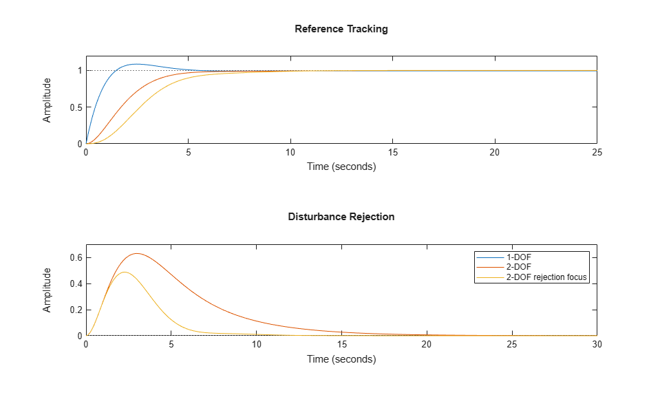
The plots show that the disturbance rejection is further improved compared to the balanced 2-DOF controller. This improvement comes with some sacrifice of reference-tracking performance, which is slightly slower. However, the reference-tracking response still has no overshoot.
Thus, using 2-DOF control can improve disturbance rejection without sacrificing as much reference tracking performance as 1-DOF control. These effects on system performance depend strongly on the properties of your plant. For some plants and some control bandwidths, using 2-DOF control or changing the design focus has less or no impact on the tuned result.