Vibration Control in Flexible Beam
This example shows how to tune a controller for reducing vibrations in a flexible beam.
Model of Flexible Beam
Figure 1 depicts an active vibration control system for a flexible beam.
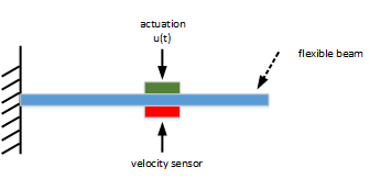
Figure 1: Active control of flexible beam
In this setup, the actuator delivering the force  and the velocity sensor are collocated. We can model the transfer function from control input to the velocity
  using finite-element analysis. Keeping only the first six modes, we obtain a plant model of the form
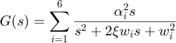
with the following parameter values.
% Parameters
xi = 0.05;
alpha = [0.09877, -0.309, -0.891, 0.5878, 0.7071, -0.8091];
w = [1, 4, 9, 16, 25, 36];
The resulting beam model for  is given by
% Beam model
G = tf(alpha(1)^2*[1,0],[1, 2*xi*w(1), w(1)^2]) + ...
    tf(alpha(2)^2*[1,0],[1, 2*xi*w(2), w(2)^2]) + ...
    tf(alpha(3)^2*[1,0],[1, 2*xi*w(3), w(3)^2]) + ...
    tf(alpha(4)^2*[1,0],[1, 2*xi*w(4), w(4)^2]) + ...
    tf(alpha(5)^2*[1,0],[1, 2*xi*w(5), w(5)^2]) + ...
    tf(alpha(6)^2*[1,0],[1, 2*xi*w(6), w(6)^2]);

G.InputName = 'uG';  G.OutputName = 'y';
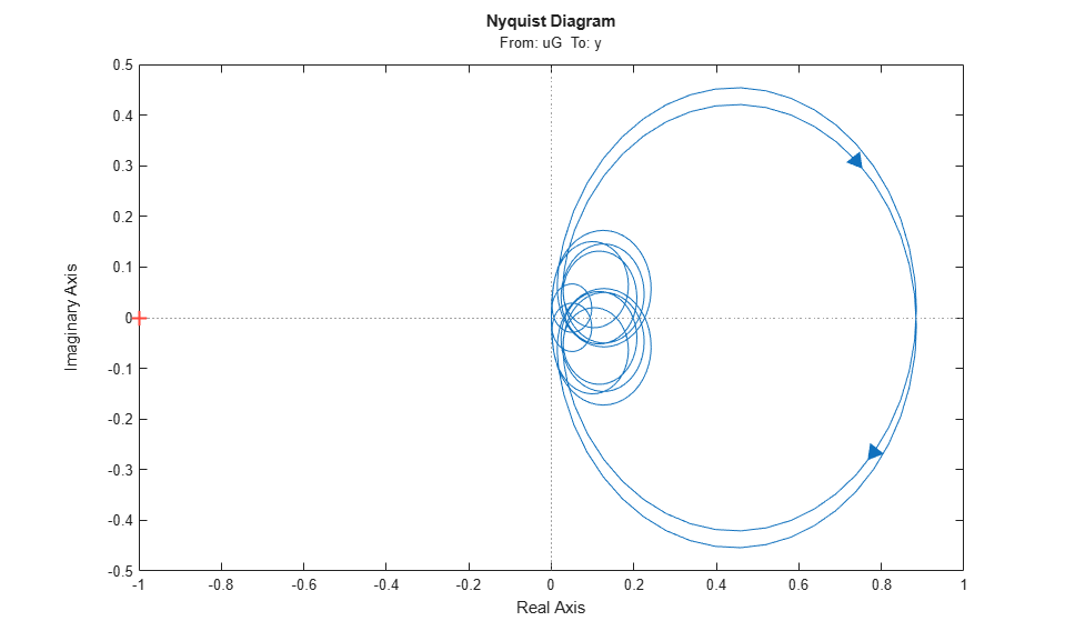
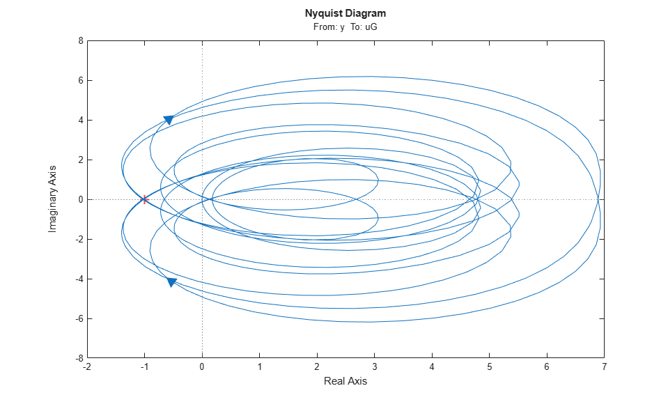
With this sensor/actuator configuration, the beam is a passive system:
isPassive(G)
ans =

  logical

   1
This is confirmed by observing that the Nyquist plot of  is positive real.
nyquist(G)
LQG Controller
LQG control is a natural formulation for active vibration control. The LQG control setup is depicted in Figure 2. The signals  and
and  are the process and measurement noise, respectively.
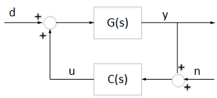
Figure 2: LQG control structure
First use lqg to compute the optimal LQG controller for the objective
with noise variances:

[a,b,c,d] = ssdata(G);
M = [c d;zeros(1,12) 1];  % [y;u] = M * [x;u]
QWV = blkdiag(b*b',1e-2);
QXU = M'*diag([1 1e-3])*M;
CLQG = lqg(ss(G),QXU,QWV);
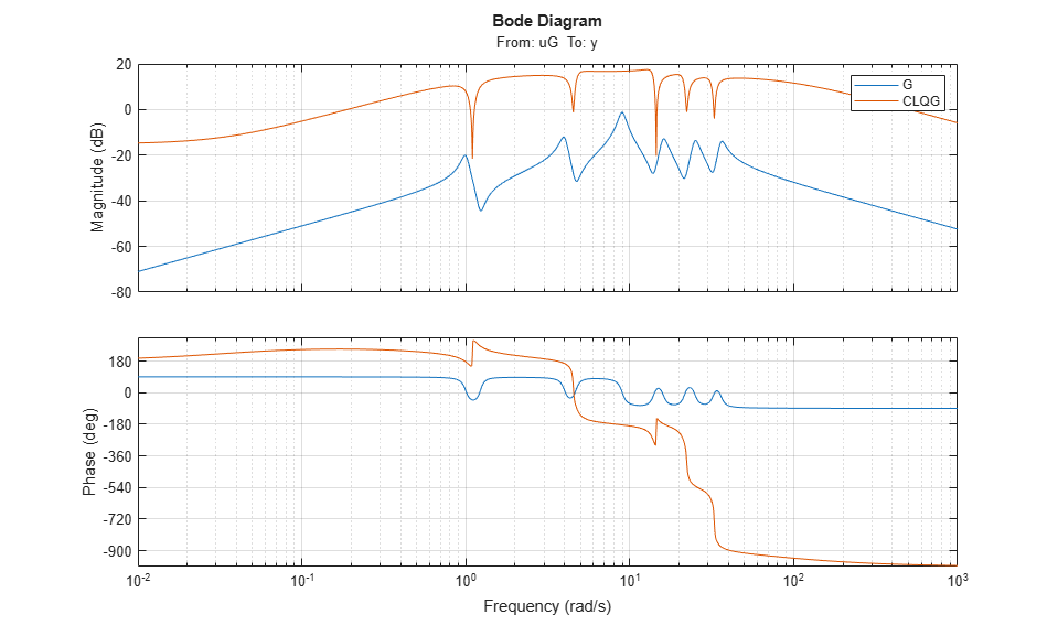
The LQG-optimal controller CLQG is complex with 12 states and several notching zeros.
size(CLQG)
State-space model with 1 outputs, 1 inputs, and 12 states.
bode(G,CLQG,{1e-2,1e3}), grid, legend('G','CLQG')
Use the general-purpose tuner systune to try and simplify this controller. With systune, you are not limited to a full-order controller and can tune controllers of any order. Here for example, let's tune a 2nd-order state-space controller.
C = ltiblock.ss('C',2,1,1);
Build a closed-loop model of the block diagram in Figure 2.
C.InputName = 'yn';  C.OutputName = 'u';
S1 = sumblk('yn = y + n');
S2 = sumblk('uG = u + d');
CL0 = connect(G,C,S1,S2,{'d','n'},{'y','u'},{'yn','u'});
Use the LQG criterion  above as sole tuning goal. The LQG tuning goal lets you directly specify the performance weights and noise covariances.
R1 = TuningGoal.LQG({'d','n'},{'y','u'},diag([1,1e-2]),diag([1 1e-3]));
Now tune the controller C to minimize the LQG objective .
[CL1,J1] = systune(CL0,R1);
Final: Soft = 0.478, Hard = -Inf, Iterations = 41
The optimizer found a 2nd-order controller with  . Compare with the optimal value for
 CLQG:
[~,Jopt] = evalGoal(R1,replaceBlock(CL0,'C',CLQG))
Jopt =

    0.4673
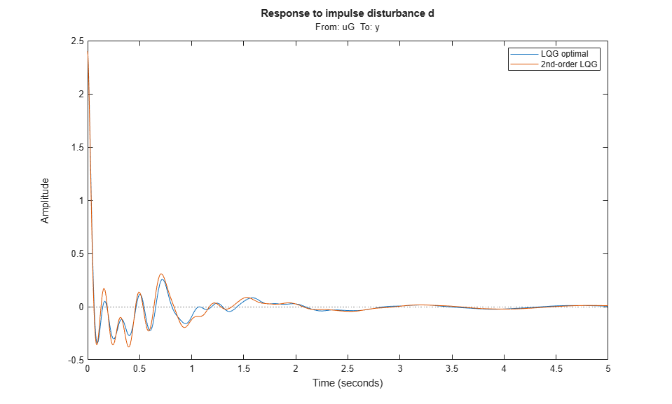
The performance degradation is less than 5%, and we reduced the controller complexity from 12 to 2 states. Further compare the impulse responses from to for the two controllers. The two responses are almost identical. You can therefore obtain near-optimal vibration attenuation with a simple second-order controller.
T0 = feedback(G,CLQG,+1);
T1 = getIOTransfer(CL1,'d','y');
impulse(T0,T1,5)
title('Response to impulse disturbance d')
legend('LQG optimal','2nd-order LQG')
Passive LQG Controller
We used an approximate model of the beam to design these two controllers. A priori, there is no guarantee that these controllers will perform well on the real beam. However, we know that the beam is a passive physical system and that the negative feedback interconnection of passive systems is always stable. So if  is passive, we can be confident that the closed-loop system will be stable.
The optimal LQG controller is not passive. In fact, its relative passive index is infinite because  is not even minimum phase.
getPassiveIndex(-CLQG)
ans =

   Inf
This is confirmed by its Nyquist plot.
nyquist(-CLQG)
Using systune, you can re-tune the second-order controller with the additional requirement that should be passive. To do this, create a passivity tuning goal for the open-loop transfer function from yn to u (which is  ). Use the "WeightedPassivity" goal to account for the minus sign.
R2 = TuningGoal.WeightedPassivity({'yn'},{'u'},-1,1);
R2.Openings = 'u';
Now re-tune the closed-loop model CL1 to minimize the LQG objective subject to being passive. Note that the passivity goal R2 is now specified as a hard constraint.
[CL2,J2,g] = systune(CL1,R1,R2);
Final: Soft = 0.478, Hard = 1, Iterations = 35
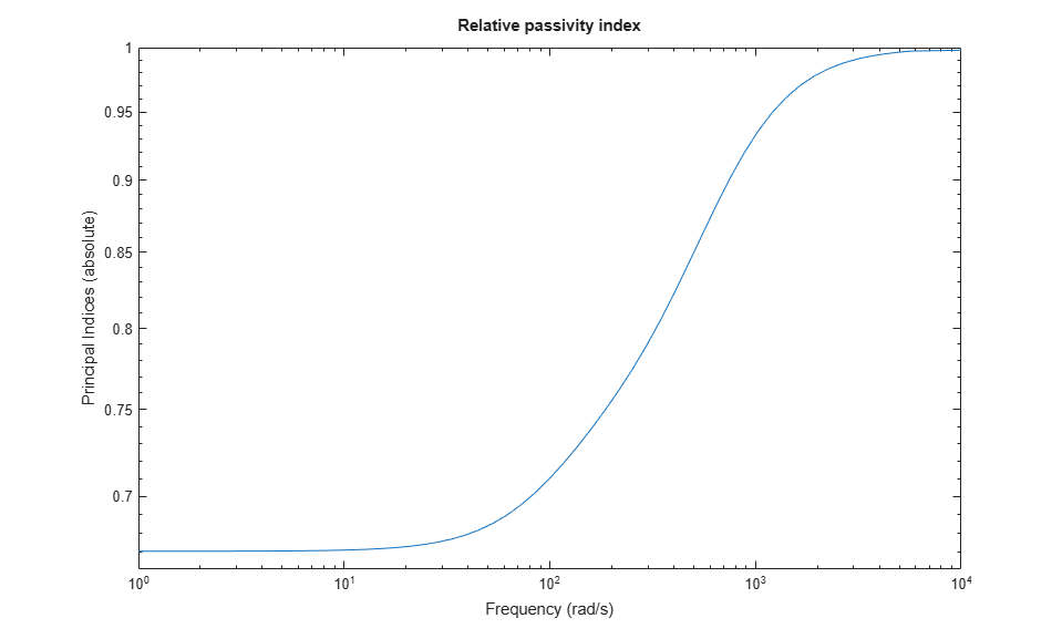
The tuner achieves the same value as previously, while enforcing passivity (hard constraint less than 1). Verify that is passive.
C2 = getBlockValue(CL2,'C');
passiveplot(-C2)
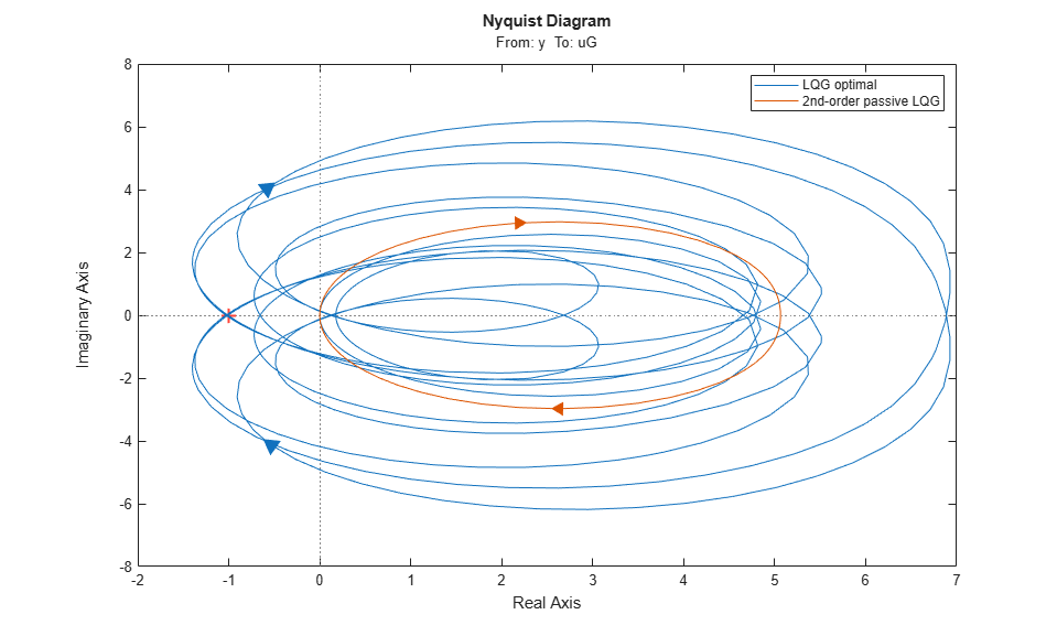
The improvement over the LQG-optimal controller is most visible in the Nyquist plot.
nyquist(-CLQG,-C2)
legend('LQG optimal','2nd-order passive LQG')
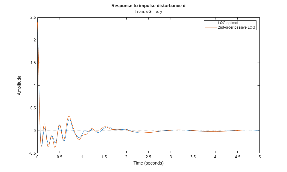
Finally, compare the impulse responses from to .
T2 = getIOTransfer(CL2,'d','y');
impulse(T0,T2,5)
title('Response to impulse disturbance d')
legend('LQG optimal','2nd-order passive LQG')
Using systune, you designed a second-order passive controller with near-optimal LQG performance.
See Also
systune | TuningGoal.WeightedPassivity | TuningGoal.LQG