Investigate Spectrogram Classifications Using LIME

This example shows how to use locally interpretable model-agnostic explanations (LIME) to investigate the robustness of a deep convolutional neural network trained to classify spectrograms. LIME is a technique for visualizing which parts of an observation contribute to the classification decision of a network. This example uses the imageLIME function to understand which features in the spectrogram data are most important for classification.

In this example, you create and train a neural network to classify four kinds of simulated time series data:

• Sine waves of a single frequency

• Superposition of three sine waves

• Broad Gaussian peaks in the time series

• Gaussian pulses in the time series

To make this problem more realistic, the time series include added confounding signals: a constant low-frequency background sinusoid and a large amount of high-frequency noise. Noisy time series data is a challenging sequence classification problem. You can approach the problem by first converting the time series data into a time-frequency spectrogram to reveal the underlying features in the time series data. You can then input the spectrograms to an image classification network.

Generate Waveforms and Spectrograms

Generate time series data for the four classes. This example uses the helper function generateSpectrogramData to generate the time series and the corresponding spectrogram data. The helper functions used in this example are attached as supporting files.

numObsPerClass = 500;

classNames = categorical(["SingleFrequency","ThreeFrequency","Gaussian","Pulse"]);
numClasses = length(classNames);

[noisyTimeSeries,spectrograms,labels] = generateSpectrogramData(numObsPerClass,classNames);

Compute the size of the spectrogram images and the number of observations.

inputSize = size(spectrograms, [1 2]);
numObs = size(spectrograms,4);

Plot Generated Data

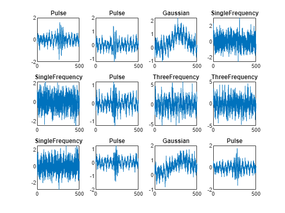
Plot a subset of the time series data with noise added. Because the noise has a comparable amplitude to the signal, the data appears noisy in the time domain. This feature makes classification a challenging problem.

figure
numPlots = 12;

for i=1:numPlots
    subplot(3,4,i)
    plot(noisyTimeSeries(i,:))
    title(labels(i))
end

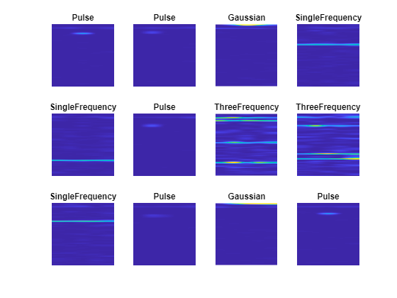
Plot the time-frequency spectrograms of the noisy data, in the same order as the time series plots. The horizontal axis is time and the vertical axis is frequency.

figure
for i=1:12
    subplot(3,4,i)
    imshow(spectrograms(:,:,1,i))
    hold on
    colormap parula
    title(labels(i))
    hold off
end

Features from each class are clearly visible, demonstrating why converting from the time domain to spectrogram images can be beneficial for this type of problem. For example, the SingleFrequency class has a single peak at the fundamental frequency, visible as a horizontal bar in the spectrogram. For the ThreeFrequency class, the three frequencies are visible.

All classes display a faint band at low frequency (near the top of the image), corresponding to the background sinusoid.

Split Data

Use the splitlabels function to divide the data into training and validation data. Use 80% of the data for training and 20% for validation.

splitIndices = splitlabels(labels,0.8);

trainLabels = labels(splitIndices{1});
trainSpectrograms = spectrograms(:,:,:,splitIndices{1});

valLabels = labels(splitIndices{2});
valSpectrograms = spectrograms(:,:,:,splitIndices{2});

Define Neural Network Architecture

Create a convolutional neural network with blocks of convolution, batch normalization, and ReLU layers.

dropoutProb = 0.2;
numFilters = 8;

layers = [
    imageInputLayer(inputSize)
    
    convolution2dLayer(3,numFilters,Padding="same")
    batchNormalizationLayer
    reluLayer    
    maxPooling2dLayer(3,Stride=2,Padding="same")
    
    convolution2dLayer(3,2*numFilters,Padding="same")
    batchNormalizationLayer
    
    convolution2dLayer(3,4*numFilters,Padding="same")
    batchNormalizationLayer
    reluLayer   
    globalMaxPooling2dLayer
    
    dropoutLayer(dropoutProb)
    fullyConnectedLayer(numClasses)
    softmaxLayer];

Define Training Options

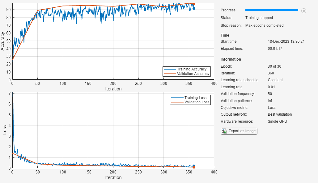
Define options for training using the SGDM optimizer. Shuffle the data every epoch by setting the 'Shuffle' option to 'every-epoch'. Monitor the training progress by setting the 'Plots' option to 'training-progress'. To suppress verbose output, set 'Verbose' to false.

options = trainingOptions("sgdm", ...
    Shuffle="every-epoch", ...
    Plots="training-progress", ...
    Verbose=false, ...
    ValidationData={valSpectrograms,valLabels}, ...
    Metrics="accuracy");

Train Network

Train the neural network using the trainnet function. For classification, use cross-entropy loss. By default, the trainnet function uses a GPU if one is available. Training on a GPU requires a Parallel Computing Toolbox™ license and a supported GPU device. For information on supported devices, see GPU Computing Requirements (Parallel Computing Toolbox). Otherwise, the trainnet function uses the CPU. To specify the execution environment, use the ExecutionEnvironment training option.

net = trainnet(trainSpectrograms,trainLabels,layers,"crossentropy",options);

Accuracy

Use the trained network to classify the validation observations using the minibatchpredict function. To convert the prediction scores to labels, use the scores2label function.

scores = minibatchpredict(net,valSpectrograms);
predLabels = scores2label(scores,categories(classNames));

Investigate the network performance by plotting a confusion matrix with confusionchart.

figure
confusionchart(valLabels,predLabels,'Normalization','row-normalized')

The network accurately classifies the validation spectrograms, with close to 100% accuracy for most of the classes.

Investigate Network Predictions

Use the imageLIME function to understand which features in the image data are most important for classification.

The LIME technique segments an image into several features and generates synthetic observations by randomly including or excluding features. Each pixel in an excluded feature is replaced with the value of the average image pixel. The network classifies these synthetic observations, and uses the resulting scores for the predicted class, along with the presence or absence of a feature, as responses and predictors to train a regression problem with a simpler model—in this example, a regression tree. The regression tree tries to approximate the behavior of the network on a single observation. It learns which features are important and significantly impact the class score.

Define Custom Segmentation Map

By default, imageLIME uses superpixel segmentation to divide the image into features. This option works well for natural images, but is less effective for spectrogram data. You can specify a custom segmentation map by setting the 'Segmentation' name-value argument to a numeric array the same size as the image, where each element is an integer corresponding to the index of the feature that pixel is in.

For the spectrogram data, the spectrogram images have much finer features in the y-dimension (frequency) than the x-dimension (time). Generate a segmentation map with 240 segments, in a 40-by-6 grid, to provide higher frequency resolution. Upsample the grid to the size of the image by using the imresize function, specifying the upsampling method as 'nearest'.

featureIdx = 1:240;
segmentationMap = reshape(featureIdx,6,40)';
segmentationMap = imresize(segmentationMap,inputSize,'nearest');

Compute LIME Map

Plot the spectrogram and compute the LIME map for two observations from each class.

obsToShowPerClass = 2;

for j=1:obsToShowPerClass
    figure

    for i=1:length(classNames)

        idx = find(valLabels == classNames(i),obsToShowPerClass);

        % Read the test image and label.
        testSpectrogram = valSpectrograms(:,:,:,idx(j));
        testLabel = valLabels(idx(j));
        testChannel = find(testLabel == categories(classNames));

        % Compute the LIME importance map.
        map = imageLIME(net,testSpectrogram,testChannel, ...
            'NumSamples',4096, ...
            'Segmentation',segmentationMap);

        % Rescale the map to the size of the image.
        mapRescale = uint8(255*rescale(map));

        % Plot the spectrogram image next to the LIME map.
        subplot(2,2,i)
        imshow(imtile({testSpectrogram,mapRescale}))
        title(string(testLabel))
        colormap parula
    end
end

The LIME maps demonstrate that for most classes, the network is focused on the relevant features for classification. For example, for the SingleFrequency class, the network focuses on the frequency corresponding to the power spectrum of the sine wave and not on spurious background details or noise.

For the SingleFrequency class, the network uses the frequency to classify. For the Pulse and Gaussian classes, the network additionally focuses on the correct frequency part of the spectrogram. For these three classes, the network is not confused by the background frequency visible near the top of all of the spectrograms. This information is not helpful for distinguishing between these classes (as it is present in all classes), so the network ignores it. In contrast, for the ThreeFrequency class, the constant background frequency is relevant to the classification decision of the network. For this class, the network does not ignore this frequency, but treats it with similar importance to the three actual frequencies.

The imageLIME results demonstrate that the network is correctly using peaks in the time-frequency spectrograms and is not confused by the spurious background sinusoid for all classes except for the ThreeFrequency class, where the network does not distinguish between the three frequencies in the signal and the low-frequency background.