Train Sequence Classification Network Using Custom Training Loop
This example shows how to train a network that classifies sequences with a custom learning rate schedule.
You can train most types of neural networks using the trainnet and trainingOptions functions. If the trainingOptions function does not provide the options you need (for example, a custom solver), then you can define your own custom training loop using dlarray and dlnetwork objects for automatic differentiation. For an example showing how to train a convolutional neural network for sequence classification using the trainnet function, see Sequence Classification Using 1-D Convolutions.
Training a network in a custom training loop with sequence data requires some additional processing steps when compared with image or feature data. Most deep learning functions require data passed as numeric arrays with a fixed sequence length. If you have sequence data where observations have varying lengths, then you must pad or truncate the sequences in each mini-batch so that they have the same length.
This example trains a network to classify sequences with the stochastic gradient descent algorithm (without momentum).
Load Training Data
Load the Waveform data set from WaveformData.mat. The observations are numTimeSteps-by-numChannels arrays, where numTimeSteps and numChannels are the number of time steps and channels of the sequence, respectively. The sequences have different lengths.
load WaveformDataView the sizes of the first few sequences.
data(1:5)
ans=5×1 cell array
    {103×3 double}
    {136×3 double}
    {140×3 double}
    {124×3 double}
    {127×3 double}
View the number of channels. To train the network, each sequence must have the same number of channels.
numChannels = size(data{1},2)numChannels = 3
Visualize the first few sequences in a plot.
figure
tiledlayout(2,2)
for i = 1:4
    nexttile
    stackedplot(data{i},DisplayLabels="Channel " + (1:numChannels));
    title("Observation " + i + newline + "Class: " + string(labels(i)))
    xlabel("Time Step")
end

Determine the number of classes in the training data.
classNames = categories(labels);
numClasses = numel(classNames);
Partition the data into training and test partitions. Train the network using the 90% of the data and set aside 10% for testing.
numObservations = numel(data);
idxTrain = 1:floor(0.9*numObservations);
XTrain = data(idxTrain);
TTrain = labels(idxTrain);

idxTest = floor(0.9*numObservations)+1:numObservations;
XTest = data(idxTest);
TTest = labels(idxTest);
Define Network
Define the network for sequence classification.
For the sequence input, specify a sequence input layer with input size matching the number of channels of the training data.
Specify three convolution-layernorm-ReLU blocks.
Pad the input to the convolution layers such that the output has the same size by setting the
Paddingoption to"same".For the first convolution layer specify 20 filters of size 5.
Pool the time steps to a single value using a 1-D global average pooling layer.
For classification, specify a fully connected layer with size matching the number of classes
To map the output to probabilities, include a softmax layer.
When training a network using a custom training loop, do not include an output layer.
layers = [
    sequenceInputLayer(numChannels)
    convolution1dLayer(5,20,Padding="same")
    layerNormalizationLayer
    reluLayer
    convolution1dLayer(5,20,Padding="same")
    layerNormalizationLayer
    reluLayer
    convolution1dLayer(5,20,Padding="same")
    layerNormalizationLayer
    reluLayer
    globalAveragePooling1dLayer
    fullyConnectedLayer(numClasses)
    softmaxLayer];
Create a dlnetwork object from the layer array.
net = dlnetwork(layers)
net =
  dlnetwork with properties:

         Layers: [13×1 nnet.cnn.layer.Layer]
    Connections: [12×2 table]
     Learnables: [14×3 table]
          State: [0×3 table]
     InputNames: {'sequenceinput'}
    OutputNames: {'softmax'}
    Initialized: 1

  View summary with summary.
Define Model Loss Function
Training a deep neural network is an optimization task. By considering a neural network as a function , where is the network input, and is the set of learnable parameters, you can optimize so that it minimizes some loss value based on the training data. For example, optimize the learnable parameters such that for a given inputs with a corresponding targets , they minimize the error between the predictions and .
Define the modelLoss function. The modelLoss function takes a dlnetwork object net, a mini-batch of input data X with corresponding targets T and returns the loss and the gradients of the loss with respect to the learnable parameters in net. To compute the gradients automatically, use the dlgradient function.
function [loss,gradients] = modelLoss(net,X,T)

% Forward data through network.
Y = forward(net,X);

% Calculate cross-entropy loss.
loss = crossentropy(Y,T);

% Calculate gradients of loss with respect to learnable parameters.
gradients = dlgradient(loss,net.Learnables);

end
Define SGD Function
Create the function sgdStep that takes the parameters and the gradients of the loss with respect to the parameters, and returns the updated parameters using the stochastic gradient descent algorithm, expressed as , where is the iteration number, is the learning rate, and denotes the gradients (the derivatives of the loss with respect to the learnable parameters).
function parameters = sgdStep(parameters,gradients,learnRate)

parameters = parameters - learnRate .* gradients;

end
Defining a custom update function is not a necessary step for custom training loops. Alternatively, you can use built in update functions like sgdmupdate, adamupdate, and rmspropupdate.
Specify Training Options
Train for 300 epochs with a mini-batch size of 128 and a learning rate of 0.05.
numEpochs = 300;
miniBatchSize = 128;
learnRate = 0.05;
Train Model
Create a minibatchqueue object that processes and manages mini-batches of data during training.
Mini-batch queue objects require data specified as datastores. Convert the sequences and labels to array datastores and combine them using the combine function. To output sequences as a cell array of numeric arrays, specify an output type of "same" for the sequence data.
adsXTrain = arrayDatastore(XTrain,OutputType="same");
adsTTrain = arrayDatastore(TTrain);
cdsTrain = combine(adsXTrain,adsTTrain);
Create a minibatchqueue object that processes and manages mini-batches of data during training. For each mini-batch:
Use the custom mini-batch preprocessing function
preprocessMiniBatch(defined at the end of this example) to pad the sequences to have the same length and convert the labels to one-hot encoded variables.Because the data has rows and columns that correspond to time steps and channels, respectively, format the sequence data with the dimension labels
"TCB"(time, channel, batch). By default, theminibatchqueueobject converts the data todlarrayobjects with underlying typesingle. Do not format the class labels.Train on a GPU if one is available. By default, the
minibatchqueueobject converts each output to agpuArrayif a GPU is available. Using a GPU requires a Parallel Computing Toolbox™ license and a supported GPU device. For information about supported devices, see GPU Computing Requirements (Parallel Computing Toolbox).
mbq = minibatchqueue(cdsTrain, ...
    MiniBatchSize=miniBatchSize, ...
    MiniBatchFcn=@preprocessMiniBatch, ...
    MiniBatchFormat=["TCB" ""]);
Calculate the total number of iterations for the training progress monitor.
numObservationsTrain = size(XTrain,1);
numIterationsPerEpoch = ceil(numObservationsTrain / miniBatchSize);
numIterations = numEpochs * numIterationsPerEpoch;
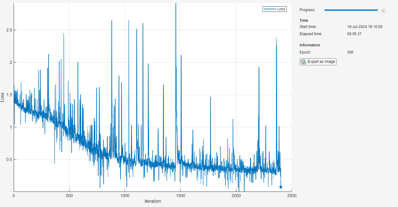
Initialize the TrainingProgressMonitor object. Because the timer starts when you create the monitor object, make sure that you create the object close to the training loop.
monitor = trainingProgressMonitor( ...
    Metrics="Loss", ...
    Info="Epoch", ...
    XLabel="Iteration");
Train the network using a custom training loop. For each epoch, shuffle the data and loop over mini-batches of data. For each mini-batch:
Evaluate the model loss and gradients using the
dlfevalandmodelLossfunctions.Update the network parameters using the
dlupdatefunction with the custom update function.Update the loss and epoch values in the training progress monitor.
Stop if the
Stopproperty of the monitor istrue. TheStopproperty value of theTrainingProgressMonitorobject changes to true when you click the Stop button.
epoch = 0;
iteration = 0;
% Loop over epochs.
while epoch < numEpochs && ~monitor.Stop

    epoch = epoch + 1;

    % Shuffle data.
    shuffle(mbq);

    % Loop over mini-batches.
    while hasdata(mbq) && ~monitor.Stop

        iteration = iteration + 1;

        % Read mini-batch of data.
        [X,T] = next(mbq);

        % Evaluate the model gradients and loss using dlfeval and the
        % modelLoss function.
        [loss,gradients] = dlfeval(@modelLoss,net,X,T);

        % Update the network parameters using SGD.
        updateFcn = @(parameters,gradients) sgdStep(parameters,gradients,learnRate);
        net = dlupdate(updateFcn,net,gradients);

        % Update the training progress monitor.
        recordMetrics(monitor,iteration,Loss=loss);
        updateInfo(monitor,Epoch=epoch);
        monitor.Progress = 100 * iteration/numIterations;
    end
end
Test Model
Test the neural network using the testnet function. For single-label classification, evaluate the accuracy. The accuracy is the percentage of correct predictions. By default, the testnet function uses a GPU if one is available. Otherwise, the function uses the CPU. To select the execution environment manually, use the ExecutionEnvironment argument of the testnet function.
accuracy = testnet(net,XTest,TTest,"accuracy")accuracy = 86
Visualize the predictions in a confusion chart. Make predictions using the minibatchpredict function, and convert the classification scores to labels using the scores2label function. By default, the minibatchpredict function uses a GPU if one is available. To select the execution environment manually, use the ExecutionEnvironment argument of the minibatchpredict function.
scores = minibatchpredict(net,XTest);
YTest = scores2label(scores,classNames);
Visualize the predictions in a confusion chart.
figure
confusionchart(TTest,YTest)

Large values on the diagonal indicate accurate predictions for the corresponding class. Large values on the off-diagonal indicate strong confusion between the corresponding classes.
Supporting Functions
Mini Batch Preprocessing Function
The preprocessMiniBatch function preprocesses a mini-batch of predictors and labels using the following steps:
Pad the sequence data in the input cell array over the first dimension (the time dimension) using the
padsequencesfunction. The function returns the data as anumTimeSteps-by-numChannels-by-numObservationsarray. To pass this information to downstream functions, specify that this data has a format of"TCB"(time, channel, batch).Extract the label data from the incoming cell array and concatenate into a categorical array along the second dimension.
One-hot encode the categorical labels into numeric arrays. Encoding into the first dimension produces an encoded array that matches the shape of the network output.
function [X,T] = preprocessMiniBatch(dataX,dataT)

% Pad sequences.
X = padsequences(dataX,1);

% Extract label data from cell and concatenate.
T = cat(2,dataT{1:end});

% One-hot encode labels.
T = onehotencode(T,1);

end
See Also
trainingProgressMonitor | dlarray | dlgradient | dlfeval | dlnetwork | forward | adamupdate | predict | minibatchqueue | onehotencode | onehotdecode
Topics
- Custom Loss Functions
- Custom Training Loops
- Custom Training Loop Model Loss Functions
- Train Generative Adversarial Network (GAN)
- Update Batch Normalization Statistics in Custom Training Loop
- Specify Training Options in Custom Training Loop
- Monitor Custom Training Loop Progress
- List of Deep Learning Layers
- List of Functions with dlarray Support