Calibrate the SABR Model Using Normal (Bachelier) Volatilities with Negative Strikes

Open Live Script

This example shows how to use two different methods to calibrate the SABR stochastic volatility model from market implied Normal (Bachelier) volatilities with negative strikes. Both approaches use normalvolbysabr, which computes the implied Normal volatilities by using the SABR model. When the Beta parameter of the SABR model is set to zero, the model is a Normal SABR model, which allows computing the implied Normal volatilities for negative strikes.

Load the Market Implied Normal (Bachelier) Volatility Data

Set up hypothetical market implied Normal volatilities for European swaptions over a range of strikes before calibration. The swaptions expire in one year from the Settle date and have two-year swaps as the underlying instrument. The rates are expressed in decimals. The market implied Normal volatilities are converted from basis points to decimals. (Changing the units affects the numerical value and interpretation of the Alpha parameter input to the function normalvolbysabr.)

% Load the market implied Normal volatility data for swaptions expiring in one year.
Settle = '20-Sep-2017';
ExerciseDate = '20-Sep-2018';
Basis = 1;

ATMStrike = -0.174/100;
MarketStrikes = ATMStrike + ((-0.5:0.25:1.5)')./100;
MarketVolatilities = [20.58 17.64 16.93 18.01 20.46 22.90 26.11 28.89 31.91]'/10000;

% At the time of Settle, define the underlying forward rate and the at-the-money volatility.
CurrentForwardValue = MarketStrikes(3)

CurrentForwardValue = -0.0017

ATMVolatility = MarketVolatilities(3)

ATMVolatility = 0.0017

Method 1: Calibrate `Alpha`, `Rho`, and `Nu` Directly

This section demonstrates how to calibrate the Alpha, Rho, and Nu parameters directly. The value of the Beta parameter is set to zero in order to allow negative rates in the SABR model (Normal SABR). After fixing the value of $β$ (Beta), the parameters $α$ (Alpha), $ρ$ (Rho), and $ν$ (Nu) are all fitted directly. The Optimization Toolbox™ function lsqnonlin generates the parameter values that minimize the squared error between the market volatilities and the volatilities computed by normalvolbysabr.

% Define the predetermined Beta
Beta1 = 0; % Setting Beta to zero allows negative rates for Normal volatilities

% Calibrate Alpha, Rho, and Nu
objFun = @(X) MarketVolatilities - ...
    normalvolbysabr(X(1), Beta1, X(2), X(3), Settle, ...
    ExerciseDate, CurrentForwardValue, MarketStrikes, 'Basis', Basis);

% If necessary, tolerances and stopping criteria can be adjusted for lsqnonlin 
X = lsqnonlin(objFun, [ATMVolatility 0 0.5], [0 -1 0], [Inf 1 Inf]);

Local minimum found.

Optimization completed because the size of the gradient is less than
the value of the optimality tolerance.

Alpha1 = X(1);
Rho1 = X(2);
Nu1 = X(3);

Method 2: Calibrate `Rho` and `Nu` by Implying `Alpha` from At-The-Money Volatility

This section demonstrates how to use an alternative calibration method where the value of $β$ is again predetermined to be zero in order to allow negative rates. However, after fixing the value of $β$ (Beta), the parameters $ρ$ (Rho), and $ν$ (Nu) are fitted directly while $α$ (Alpha) is implied from the market at-the-money volatility. Models calibrated using this method produce at-the-money volatilities that are equal to market quotes. This approach can be useful when at-the-money volatilities are quoted most frequently and are important to match. In order to imply $α$ (Alpha) from market at-the-money Normal volatility ( $σ_{N o r m a l, A T M}$ ), the following cubic polynomial is solved for $α$ (Alpha), and the smallest positive real root is selected. This is similar to the approach used for implying $α$ (Alpha) from market at-the-money Black volatility [2]. However, note that the following expression that is used for Normal volatilities is different from another expression that is used for Black volatilities.

$\frac{β (β - 2) T}{24 F^{(2 - 2 β)}} α^{3} + \frac{ρ β ν T}{4 F^{(1 - β)}} α^{2} + (1 + \frac{2 - 3 ρ^{2}}{24} ν^{2} T) α - σ_{N o r m a l, A T M} F^{- β} = 0$

% Define the predetermined Beta
Beta2 = 0; % Setting Beta to zero allows negative rates for Normal volatilities

% Year fraction from Settle to option maturity
T = yearfrac(Settle, ExerciseDate, Basis);

% This function solves the SABR at-the-money volatility equation as a
% polynomial of Alpha
alpharootsNormal = @(Rho,Nu) roots([...
    Beta2.*(Beta2 - 2)*T/24/CurrentForwardValue^(2 - 2*Beta2) ...
    Rho*Beta2*Nu*T/4/CurrentForwardValue^(1 - Beta2) ...
    (1 + (2 - 3*Rho^2)*Nu^2*T/24) ...
    -ATMVolatility*CurrentForwardValue^(-Beta2)]);

% This function converts at-the-money volatility into Alpha by picking the
% smallest positive real root 
atmNormalVol2SabrAlpha = @(Rho,Nu) min(real(arrayfun(@(x) ...
    x*(x>0) + realmax*(x<0 || abs(imag(x))>1e-6), alpharootsNormal(Rho,Nu))));

% Calibrate Rho and Nu (while converting at-the-money volatility into Alpha
% using atmVol2NormalSabrAlpha)
objFun = @(X) MarketVolatilities - ...
    normalvolbysabr(atmNormalVol2SabrAlpha(X(1), X(2)), ...
    Beta2, X(1), X(2), Settle, ExerciseDate, CurrentForwardValue, ...
    MarketStrikes, 'Basis', Basis);

% If necessary, tolerances and stopping criteria can be adjusted for lsqnonlin 
X = lsqnonlin(objFun, [0 0.5], [-1 0], [1 Inf]);

Local minimum found.

Optimization completed because the size of the gradient is less than
the value of the optimality tolerance.

Rho2 = X(1);
Nu2 = X(2);

% Obtain final Alpha from at-the-money volatility using calibrated parameters
Alpha2 = atmNormalVol2SabrAlpha(Rho2, Nu2);

% Display calibrated parameters
C = {Alpha1 Beta1 Rho1 Nu1;Alpha2 Beta2 Rho2 Nu2};
format;
CalibratedPrameters = cell2table(C,...
    'VariableNames',{'Alpha' 'Beta' 'Rho' 'Nu'},...
    'RowNames',{'Method 1';'Method 2'})

CalibratedPrameters=2×4 table
                  Alpha      Beta       Rho         Nu   
                _________    ____    _________    _______

    Method 1    0.0016332     0      -0.034233    0.45877
    Method 2    0.0016652     0        -0.0318    0.44812

Use the Calibrated Models

Use the calibrated models to compute new volatilities at any strike value, including negative strikes.

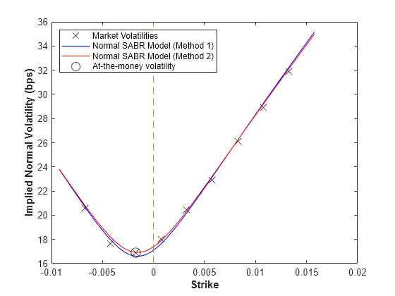
Compute volatilities for models calibrated using Method 1 and Method 2, then plot the results. The model calibrated using Method 2 reproduces the market at-the-money volatility (marked with a circle) exactly.

PlottingStrikes = (min(MarketStrikes)-0.0025:0.0001:max(MarketStrikes)+0.0025)';

% Compute volatilities for model calibrated by Method 1
ComputedVols1 = normalvolbysabr(Alpha1, Beta1, Rho1, Nu1, Settle, ...
    ExerciseDate, CurrentForwardValue, PlottingStrikes, 'Basis', Basis);

% Compute volatilities for model calibrated by Method 2
ComputedVols2 = normalvolbysabr(Alpha2, Beta2, Rho2, Nu2, Settle, ...
    ExerciseDate, CurrentForwardValue, PlottingStrikes, 'Basis', Basis);

figure;
plot(MarketStrikes,MarketVolatilities*10000,'xk',...
    PlottingStrikes,ComputedVols1*10000,'b', ...  
    PlottingStrikes,ComputedVols2*10000,'r', ...
    CurrentForwardValue,ATMVolatility*10000,'ok',...
    'MarkerSize',10);

h = gca;
line([0,0],[min(h.YLim),max(h.YLim)],'LineStyle','--');

xlabel('Strike', 'FontWeight', 'bold');
ylabel('Implied Normal Volatility (bps)', 'FontWeight', 'bold');
legend('Market Volatilities', 'Normal SABR Model (Method 1)', ...
    'Normal SABR Model (Method 2)', 'At-the-money volatility', ...
    'Location', 'northwest');

References

[1] Hagan, P. S., Kumar, D., Lesniewski, A. S. and Woodward, D. E. "Managing smile risk." Wilmott Magazine, 2002.

[2] West, G. "Calibration of the SABR Model in Illiquid Markets." Applied Mathematical Finance, 12(4), pp. 371–385, 2004.

Calibrate the SABR Model Using Normal (Bachelier) Volatilities with Negative Strikes

Load the Market Implied Normal (Bachelier) Volatility Data

Method 1: Calibrate Alpha, Rho, and Nu Directly

Method 2: Calibrate Rho and Nu by Implying Alpha from At-The-Money Volatility

Use the Calibrated Models

References

Related Topics

Method 1: Calibrate `Alpha`, `Rho`, and `Nu` Directly

Method 2: Calibrate `Rho` and `Nu` by Implying `Alpha` from At-The-Money Volatility