Tracking with Range-Only Measurements
This example illustrates the use of particle filters and Gaussian-sum filters to track a single object using range-only measurements.
Introduction
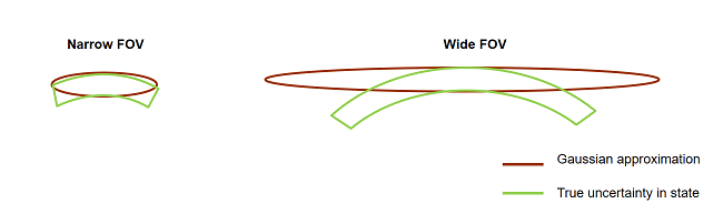
Sensors that can only observe range information cannot provide a complete understanding of the object's state from a single detection. In addition, the uncertainty of a range-only measurement, when represented in a Cartesian coordinate frame, is non-Gaussian and creates a concave shape. For range-only sensors with a narrow field of view (FOV), the angular uncertainty is small and can be approximated by an ellipsoid, that is, a Gaussian distribution. However, for range-only sensors with a wide FOV, the uncertainty, when represented in a Cartesian frame, is described by a concave ring shape, which cannot be easily approximated by an ellipsoid. This is illustrated in the image shown below.
This phenomenon is also observed with long-range radars, which provide both azimuth and range information. When the FOV of each azimuth resolution cell spans a large region in space, the distribution of state becomes non-Gaussian. Techniques like long-range corrections are often employed to make use of Gaussian filters like extended Kalman filters (trackingEKF) and Unscented Kalman filters (trackingUKF) in those scenarios. This is demonstrated in detail in the Multiplatform Radar Detection Fusion example.
In this example, you will learn how to use a particle filter and a Gaussian-sum filter to represent the non-Gaussian uncertainty in state caused by range measurements from large FOV sensors.
Define Scenario
The scenario models a single object traveling at a constant velocity in the X-Y plane. The object crosses through the coverage areas of three equally spaced sensors, with FOV of 60 degrees in azimuth. The sensors FOV overlap, which enhances observability when the object crosses through the overlapping regions. Each sensor reports range measurement with a measurement accuracy of 5 centimeters.
s = rng;
rng(2018);
[scene,theaterDisplay] = helperCreateRangeOnlySensorScenario;
showScenario(theaterDisplay)
![]()
showGrabs(theaterDisplay,[]);
Track Using a Particle Filter
In this section, a particle filter, trackingPF is used to track the object. The tracking is performed by a single-hypothesis tracker using trackerGNN. The tracker is responsible for maintaining the track while reducing the number of false alarms.
The function initRangeOnlyCVPF initializes a constant velocity particle filter. The function is similar to the initcvpf function, but limits the angles from [-180 180] in azimuth and [-90 90] in elevation for initcvpf to the known sensor FOV in this problem.
% Tracker
tracker = trackerGNN('FilterInitializationFcn',@initRangeOnlyCVPF,'MaxNumTracks',5);

% Update display to plot particle data
theaterDisplay.FilterType = 'trackingPF';

% Advance scenario and track object
while advance(scene)
    % Current time
    time = scene.SimulationTime;

    % Generate detections
    [detections, configs] = generateRangeDetections(scene);

    % Pass detections to tracker
    if ~isempty(detections)
        [confTracks,~,allTracks] = tracker(detections,time);
    elseif isLocked(tracker)
        confTracks = predictTracksToTime(tracker,'confirmed',time);
    end

    % Update display
    theaterDisplay(detections,configs,confTracks,tracker);
end
Notice that the particles carry a non-Gaussian uncertainty in state along the arc of range-only measurement till the target gets detected by the next sensor. As the target moves through the boundaries of the sensor coverage areas, the likelihood of particles at the boundary increases as compared to other particles. This increase in likelihood triggers a resampling step in the particle filter and the particles collapse to the true target location.
showGrabs(theaterDisplay,[1 2]);
![]()
![]()
Using the particle filter, the tracker maintains the track for the duration of the scenario.
showGrabs(theaterDisplay,3);
![]()
Track Using a Gaussian-Sum Filter
In this section, a Gaussian-sum filter, trackingGSF, is used to track the object. For range-only measurements, you can initialize a trackingGSF using initapekf. The initapekf function initializes an angle-parameterized extended Kalman filter. The function initRangeOnlyGSF defined in this example modifies the initapekf function to track slow moving objects.
% restart scene
restart(scene);
release(theaterDisplay);

% Tracker
tracker = trackerGNN('FilterInitializationFcn',@initRangeOnlyGSF);

% Update display to plot Gaussian-sum components
theaterDisplay.FilterType = 'trackingGSF';

while advance(scene)
    % Current time
    time = scene.SimulationTime;

    % Generate detections
    [detections, configs] = generateRangeDetections(scene);

    % Pass detections to tracker
    if ~isempty(detections)
        [confTracks,~,allTracks] = tracker(detections,time);
    elseif isLocked(tracker)
        confTracks = predictTracksToTime(tracker,'confirmed',time);
    end

    % Update display
    theaterDisplay(detections,configs,confTracks,tracker);
end
You can use the TrackingFilters property of the trackingGSF to see the state of each extended Kalman filter. Represented by "Individual Filters" in the next figure, notice how the filters are aligned along the arc generated by range-only measurement until the target reaches the overlapping region. Immediately after crossing the boundary, the likelihood of the filter at the boundary increases and the track converges to that individual filter. The weight, ModelProbabilities, of other individual filters drop as compared to the one closest to the boundary, and their contribution to the estimation of state reduces.
showGrabs(theaterDisplay,[4 5]);
![]()
![]()
Using the Gaussian-sum filter, the tracker maintains the track during for the duration of the scenario.
showGrabs(theaterDisplay,6);
rng(s)
![]()
Summary
In this example, you learned how to use a particle filter and a Gaussian-sum filter to track an object using range-only measurements. Both particle filters and Gaussian-sum filters offer capabilities to track objects that follow a non-Gaussian state distribution. While the Gaussian-sum filter approximates the distribution by a weighted sum of Gaussian-components, a particle filter represents this distribution by a set of samples. The particle filter offers a more natural approach to represent any arbitrary distribution as long as samples can be generated from it. However, to represent the distribution perfectly, a large number of particles may be required, which increases computational requirements of using the filter. As state is described by samples, a particle filter architecture allows using any process noise distribution as well as measurement noise. In contrast, the Gaussian-sum filter uses a Gaussian process and measurement noise for each component. One of the major shortcoming of particles is the problem of "sample impoverishment". After resampling, the particles may collapse to regions of high likelihood, not allowing the filter to recover from an "incorrect" association. As no resampling is performed in Gaussian-sum filter and each state is Gaussian, the Gaussian-sum filters offers some capability to recover from such an association. However, this recovery is often dependent on the weights and covariances of each Gaussian-component.
Supporting Functions
generateRangeDetections This function generates range-only detection
function [detections,config] = generateRangeDetections(scene)
detections = [];
config = [];
time = scene.SimulationTime;
for i = 1:numel(scene.Platforms)
    [thisDet, thisConfig] = detectOnlyRange(scene.Platforms{i},time);
    config = [config;thisConfig]; %#ok<AGROW>
    detections = [detections;thisDet]; %#ok<AGROW>
end
end
detectOnlyRange This function remove az and el from a spherical detection
function [rangeDetections,config] = detectOnlyRange(observer,time)
    [fullDetections,numDetections,config] = detect(observer,time);
    for i = 1:numel(config)
        % Populate the config correctly for plotting
        config(i).FieldOfView = observer.Sensors{i}.FieldOfView;
        config(i).MeasurementParameters(1).OriginPosition = observer.Sensors{i}.MountingLocation(:);
        config(i).MeasurementParameters(1).Orientation = rotmat(quaternion(observer.Sensors{i}.MountingAngles(:)','eulerd','ZYX','frame'),'frame');
        config(i).MeasurementParameters(1).IsParentToChild = true;
    end

    % Remove all except range information
    rangeDetections = fullDetections;
    for i = 1:numDetections
        rangeDetections{i}.Measurement = rangeDetections{i}.Measurement(end);
        rangeDetections{i}.MeasurementNoise = rangeDetections{i}.MeasurementNoise(end);
        rangeDetections{i}.MeasurementParameters(1).HasAzimuth = false;
        rangeDetections{i}.MeasurementParameters(1).HasElevation = false;
    end
end
initRangeOnlyGSF This function initializes an angle-parameterized Gaussian-sum filter. It uses angle limits of [-30 30] to specify FOV and sets the number of filters as 10. It also modifies the state covariance and process noise for slow moving object in 2-D.
function filter = initRangeOnlyGSF(detection)
filter = initapekf(detection,10,[-30 30]);
for i = 1:numel(filter.TrackingFilters)
    filterK = filter.TrackingFilters{i};
    filterK.ProcessNoise = 0.01*eye(3);
    filterK.ProcessNoise(3,3) = 0;
    % Small covariance for slow moving targets
    filterK.StateCovariance(2,2) = 0.1;
    filterK.StateCovariance(4,4) = 0.1;
    % Low standard deviation in z as v = 0;
    filterK.StateCovariance(6,6) = 0.01;
end
end
initRangeOnlyCVPF This function initializes a constant velocity particle filter with particles limited to the FOV of [-30 30].
function filter = initRangeOnlyCVPF(detection)
filter = initcvpf(detection);

% Uniform az in FOV
az = -pi/6 + pi/3*rand(1,filter.NumParticles);
% no elevation;
el = zeros(1,filter.NumParticles);
% Samples of range from Gaussian range measurement
r = detection.Measurement + sqrt(detection.MeasurementNoise)*randn(1,filter.NumParticles);

% x,y,z in sensor frame
[x,y,z] = sph2cart(az,el,r);

% Rotate from sensor to scenario frame.
senToPlat = detection.MeasurementParameters(1).Orientation';
senPosition = detection.MeasurementParameters(1).OriginPosition;
platToScenario = detection.MeasurementParameters(2).Orientation';
platPosition = detection.MeasurementParameters(2).OriginPosition;
posPlat = senToPlat*[x;y;z] + senPosition;
posScen = platToScenario*posPlat + platPosition;

% Position particles
filter.Particles(1,:) = posScen(1,:);
filter.Particles(3,:) = posScen(2,:);
filter.Particles(5,:) = posScen(3,:);

% Velocity particles
% uniform distribution
filter.Particles([2 4],:) = -1 + 2*rand(2,filter.NumParticles);

% Process Noise is set to a low number for slow moving targets. Larger than
% GSF to add more noise to particles preventing them from collapsing.
filter.ProcessNoise = 0.1*eye(3);

% Zero z-velocity
filter.Particles(6,:) = 0;
filter.ProcessNoise(3,3) = 0;
end