Track Vehicles Using Lidar Data in Simulink
This example shows you how to track vehicles using measurements from a lidar sensor mounted on top of an ego vehicle. Due to high resolution capabilities of the lidar sensor, each scan from the sensor contains a large number of points, commonly known as a point cloud. The example illustrates the workflow in Simulink for processing the point cloud and tracking the objects. The lidar data used in this example is recorded from a highway driving scenario. You use the recorded data to track vehicles with a joint probabilistic data association (JPDA) tracker and an interacting multiple model (IMM) approach. The example closely follows the Track Vehicles Using Lidar: From Point Cloud to Track List MATLAB® example.
Setup
The lidar data used in this example is available at the following link: https://ssd.mathworks.com/supportfiles/lidar/data/TrackVehiclesUsingLidarExampleData.zip
Download the data files into the current working folder. If you want to place the files in a different folder, change the directory name in the subsequent instructions.
% Load the data if unavailable.
if ~exist('lidarData_1.mat','file')
    dataUrl = 'https://ssd.mathworks.com/supportfiles/lidar/data/TrackVehiclesUsingLidarExampleData.zip';
    datasetFolder = fullfile(pwd);
    unzip(dataUrl,datasetFolder);
end
Overview of the Model
load_system('TrackVehiclesSimulinkExample');
set_param('TrackVehiclesSimulinkExample','SimulationCommand','update');
open_system('TrackVehiclesSimulinkExample');

Lidar and Image Data Reader
The Lidar Data Reader and Image Data Reader blocks are implemented using a MATLAB System (Simulink) block. The code for the blocks is defined by helper classes, HelperLidarDataReader and HelperImageDataReader respectively. The image and lidar data readers read the recorded data from the MAT files and output the reference image and the locations of points in the point cloud respectively.
Bounding Box Detector
As described earlier, the raw data from sensor contains a large number of points. This raw data must be preprocessed to extract objects of interest, such as cars, cyclists, and pedestrian. The preprocessing is done using the Bounding Box Detector block. The Bounding Box Detector is also implemented as a MATLAB System™ block defined by a helper class, HelperBoundingBoxDetectorBlock. It accepts the point cloud locations as an input and outputs bounding box detections corresponding to obstacles. The diagram shows the processes involved in the bounding box detector model and the Computer Vision Toolbox™ functions used to implement each process. It also shows the parameters of the block that control each process.

The block outputs the detections and segmentation information as Simulink.Bus (Simulink) objects named detectionBus and segmentationBus. These buses are created in the base workspace using helper function helperCreateDetectorBus specified in the PreLoadFcn callback. See Model Callbacks (Simulink) for more information about callback functions.
Tracking algorithm
The tracking algorithm is implemented using the joint probabilistic data association (JPDA) tracker, which uses an interacting multiple model (IMM) approach to track targets. The IMM filter is implemented by the helperInitIMMFilter, which is specified as the "Filter initialization function" parameter of the block. In this example, the IMM filter is configured to use two models, a constant velocity cuboid model and a constant turn-rate cuboid model. The models define the dimensions of the cuboid as constants during state-transition and their estimates evolve in time during correction stages of the filter. The animation below shows the effect of mixing the constant velocity and constant turn-rate models with different probabilities during prediction stages of the filter.

The IMM filter automatically computes the probability of each model when the filter is corrected with detections. The animation below shows the estimated trajectory and the probability of models during a lane change event.

For a detailed description of the state transition and measurement models, refer to the "Target State and Sensor Measurement Model" section of the MATLAB example.
The tracker block selects the check box "Enable all tracks output" and "Enable detectable track IDs input" to output all tracks from the tracker and calculate their detection probability as a function of their state.
Calculate Detectability
The Calculate Detectability block is implemented using a MATLAB Function (Simulink) block. The block calculates the Detectable TrackIDs input for the tracker and outputs it as an array with 2 columns. The first column represents the TrackIDs of the tracks and the second column specifies their probability of detection by the sensor and bounding box detector.
Visualization
The Visualization block is also implemented using the MATLAB System block and is defined using HelperLidarExampleDisplayBlock. The block uses RunTimeObject parameter of the blocks to display their outputs. See Access Block Data During Simulation (Simulink) for further information on how to access block outputs during simulation.
Detections and Tracks Bus Objects
As described earlier, the inputs and outputs of different blocks are defined by bus objects. You can visualize the structure of each bus using the Type Editor (Simulink). The following images show the structure of the bus for detections and tracks.
Detections
The detectionBus outputs a nested bus object with 2 elements, NumDetections and Detections.
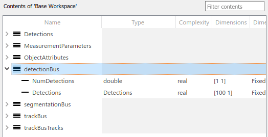
The first element, NumDetections, represents the number of detections. The second element Detections is a bus object of a fixed size representing all detections. The first NumDetections elements of the bus object represent the current set of detections. Notice that the structure of the bus is similar to the objectDetection class.

Tracks
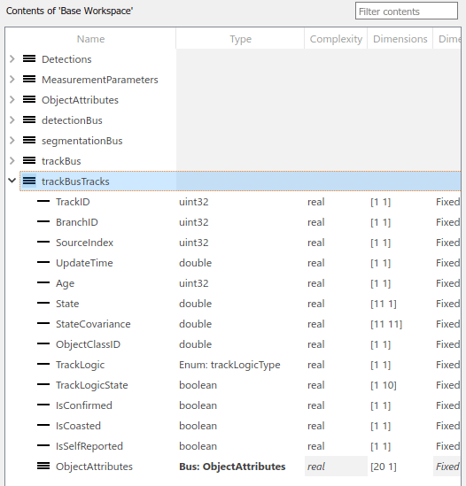
The track bus is similar to the detections bus. It is a nested bus, where NumTracks defines the number of tracks in the bus and Tracks define a fixed size of tracks. The size of the tracks is governed by the block parameter "Maximum number of tracks".

The second element Tracks is a bus object defined by trackBusTracks. This bus is automatically created by the tracker block by using the bus name specified as the prefix. Notice that the structure of the bus is similar to the objectTrack class.
Results
The detector and tracker algorithm is configured exactly as the Track Vehicles Using Lidar: From Point Cloud to Track List MATLAB example. After running the model, you can visualize the results on the figure. The animation below shows the results from time 0 to 4 seconds. The tracks are represented by green bounding boxes. The bounding box detections are represented by orange bounding boxes. The detections also have orange points inside them, representing the point cloud segmented as obstacles. The segmented ground is shown in purple. The cropped or discarded point cloud is shown in blue. Notice that the tracked objects are able to maintain their shape and kinematic center by positioning the detections onto visible portions of the vehicles. This illustrates the offset and shrinkage effect modeled in the measurement functions.
![]()
close_system('TrackVehiclesSimulinkExample');
Summary
This example showed how to use a JPDA tracker with an IMM filter to track objects using a lidar sensor. You learned how a raw point cloud can be preprocessed to generate detections for conventional trackers, which assume one detection per object per sensor scan. You also learned how to use a cuboid model to describe the extended objects being tracked by the JPDA tracker.