Wide Area Surveillance Using Ground and Airborne Radars
This example shows you how to track aircraft in an airspace using a multiplatform radar network consisting of both ground-based and airborne radars. In this example, you configure and run a Joint Integrated Probabilistic Data Association (JIPDA) tracker for wide area surveillance using recorded radar data.
Introduction
Wide area surveillance involves the continuous monitoring of large geographic regions to maintain situational awareness, particularly in the airspace. This type of surveillance introduces additional challenges for multi-object tracking due to the curvature of the Earth. From a target modeling perspective, tracking algorithms must account for the fact that a target's motion characteristics in earth-centered frame are dependent on its position on the Earth. This is due to varying directions of gravitational vector, and thus the horizontal and vertical planes.From a sensor modeling perspective, the curvature of the Earth affects the sensor's line-of-sight and detection capabilities. Additionally, coordinate systems must be defined and managed carefully, as sensor and platform data are typically provided in geo-referenced frames such as north-east-down (NED) or east-north-up (ENU).
The task-oriented framework provided by the toolbox enables you to address these challenges effectively, even without deep expertise in tracking algorithms. It offers a high-level workflow that guides you through configuring and executing a tracking system in five structured steps.
Step 1 - Specify what you want to track
In this step, you specify the type and the characteristics of the objects you intend to track. This step informs the tracker about choosing appropriate models and their parameters to define the target. You use the trackerTargetSpec function to achieve this. The function uses a library of prebuilt specifications provided in the toolbox. To check the complete library of target specifications, refer to the documentation of trackerTargetSpec function.
In this example, you define the target specification for passenger aircraft. The display below shows the list of properties of the passenger specification, which can be modified for your application. You set the IsGeographic property of the spec to true to model the impact of Earth's curvature on target motion. You also set the geographic reference frame to NED to define that the estimated velocity of the target should be with respect to NED frame at the current estimated location of the target. Under this configuration, the tracker outputs the estimate state of the object as where represents the position in earth-centered earth-fixed (ECEF) frame, and represents the velocity of the object in the local NED frame at the current estimated position.
targetSpec = trackerTargetSpec('aerospace','aircraft','passenger');
targetSpec.IsGeographic = true;
targetSpec.GeographicReferenceFrame = "NED";
disp(targetSpec)
  PassengerAircraft with properties:

                 IsGeographic: 1
     GeographicReferenceFrame: "NED"
           MaxHorizontalSpeed: 250      m/s
             MaxVerticalSpeed: 20       m/s
    MaxHorizontalAcceleration: 10       m/s²
      MaxVerticalAcceleration: 1        m/s²
Step 2 - Specify what sensors you have
In this step, you provide a detailed description of the sensors that will be employed for tracking. This step informs the tracker about choosing appropriate models and their parameters to define the sensor.
Similar to target specifications, the toolbox also provides a prebuilt library of commonly used sensors for tracking. To check the complete library of sensor specifications, refer to the trackerSensorSpec function. In this example, you will use data from five radar sensors. Three of these radar sensors are ground-based radars, and two radars are airborne radars mounted on moving platforms. The table below shows the list of radars as well as the geo-referenced frames used by each radar.
Radar | Platform LLA | Geo-reference frame for platform pose and kinematics | Platform rotation w.r.t reference frame |
Ground-based | [41.4228 -88.0583 100] | Fixed NED | yaw = 30, pitch = 0, roll = 0 |
Ground-based | [40.6989 -89.8258 100] | Fixed ENU | yaw = -15, pitch = 0, roll = 0 |
Ground-based | [39.2219 -95.2461 100] | Fixed NED | yaw = 10, pitch = 0, roll = 0 |
Airborne | Time-varying | Local ENU at current platform location | Time-varying |
Airborne | Time-varying | Local ENU at current platform location | Time-varying |
% Platform LLAs of ground radars
lat = [41.4228 40.6989 39.2219];
long = [-88.0583 -89.8258 -95.2461];
alt = [100 100 100];

% Reference frames of ground-based radars
refFrames = ["NED","ENU","NED"];

% Orientations of each ground-based platform
yaw = [30;-15;10];
pitch = [0;0;0];
roll = [0;0;0];
platformOrient = rotmat(quaternion([yaw pitch roll],'eulerd','ZYX','frame'),'frame');
To specify radar sensors in a geo-referenced environment, you will create a specification for the aerospace radar in a geo-referenced environment.Creating a geo-referenced sensor allows you to
Specify the position of the platform using geodetic coordinates (latitude, longitude, altitude)
Specify the orientation of the platform using a geo-referenced frame such as NED or ENU at the current platform location.
Model the impact of Earth's curvature on a sensor's ability to detect a target. This helps the tracker understand which targets are detectable by which sensors at any given time.
Define Specification for Ground-based Radars
To specify a geo-referenced ground-based radar, you create the sensor specification using trackerSensorSpec function and set IsGeographic property to true. You also set the IsPlatformStationary property to true to define that the sensor is a ground-based stationary radar. Next, you define platform data as well as characteristics of each radar such as its field of view, resolutions and so on.
% Allocate specifications for each ground radar as a cell
numGroundRadars = numel(lat);
groundRadarSpecs = cell(1,numGroundRadars);

% Fill in the specifications
for i = 1:numGroundRadars
    % Create geo-referenced ground-based radar
    groundRadar = trackerSensorSpec('aerospace','radar','monostatic');
    groundRadar.IsGeographic = true;
    groundRadar.IsPlatformStationary = true;

    % Define the reference frame for platform data
    groundRadar.GeographicReferenceFrame = refFrames(i);

    % Define the platform pose using geo-referenced data
    groundRadar.PlatformPosition = [lat(i) long(i) alt(i)];
    groundRadar.PlatformOrientation = platformOrient(:,:,i);

    % The radar is mounted at the center of the platform with radar axes
    % aligned with platform axes.
    groundRadar.MountingLocation = [0 0 0];
    groundRadar.MountingAngles = [0 0 0];

    % Maximum number of look angles from the radar per update to the tracker
    groundRadar.MaxNumLooksPerUpdate = 1;

    % Maximum number of measurements reported per update to the tracker
    groundRadar.MaxNumMeasurementsPerUpdate = 10;

    % Radar characteristics
    groundRadar.FieldOfView = [30 20];
    groundRadar.RangeLimits = [0 463e3];
    groundRadar.RangeRateLimits = [-500 500];
    groundRadar.ElevationResolution = 2.2275;
    groundRadar.AzimuthResolution = 1.4;
    groundRadar.RangeResolution = 323;
    groundRadar.RangeRateResolution = 100;
    groundRadar.DetectionProbability = 0.95;
    groundRadar.FalseAlarmRate = 1e-6;

    % Assign to ground radar specs
    groundRadarSpecs{i} = groundRadar;
end
Define Specification for Airborne Radars
In this section, you define the sensor specifications for the two airborne radars. To define airborne radars, you set the IsPlatformStationary property to false to indicate a moving platform. You indicate that platform's pose and kinematics will be provided with respect to local ENU frame defined at the platform's current location.
% Create airborne radar spec using an aerospace monostatic radar
numAirborneRadars = 2;
airborneRadarSpecs = cell(1, numAirborneRadars);

for i = 1:numAirborneRadars
    airborneRadar = trackerSensorSpec('aerospace','radar','monostatic');
    airborneRadar.IsGeographic = true;
    airborneRadar.GeographicReferenceFrame = "ENU";
    airborneRadar.IsPlatformStationary = false;
    airborneRadar.MaxNumLooksPerUpdate = 1;
    airborneRadar.MaxNumMeasurementsPerUpdate = 10;
    airborneRadar.MountingLocation = [0 0 0];
    airborneRadar.MountingAngles = [0 0 0];
    airborneRadar.FieldOfView = [30 20];
    airborneRadar.RangeLimits = [0 463e3];
    airborneRadar.RangeRateLimits = [-5000 5000];
    airborneRadar.ElevationResolution = 2.2275;
    airborneRadar.AzimuthResolution = 1.4;
    airborneRadar.RangeResolution = 323;
    airborneRadar.RangeRateResolution = 10;
    airborneRadar.DetectionProbability = 0.95;
    airborneRadarSpecs{i} = airborneRadar;
end
You collect all these sensor specifications in a cell array to define all the sensors used with the tracker.
sensorSpecs = [groundRadarSpecs airborneRadarSpecs];
Step 3 - Configure the tracker
In this step, you use the defined target and sensor specifications to configure a multi-object JIPDA tracker using the multiSensorTargetTracker function. The tracker uses target and sensor specifications to infer all the target and sensor models to be used for track estimation.
tracker = multiSensorTargetTracker(targetSpec, sensorSpecs, 'jipda');
disp(tracker)
fusion.tracker.JIPDATracker with properties:
TargetSpecifications: {[1×1 PassengerAircraft]}
SensorSpecifications: {[1×1 AerospaceMonostaticRadar] [1×1 AerospaceMonostaticRadar] [1×1 AerospaceMonostaticRadar] [1×1 AerospaceMonostaticRadar] [1×1 AerospaceMonostaticRadar]}
MaxMahalanobisDistance: 5
ConfirmationExistenceProbability: 0.9000
DeletionExistenceProbability: 0.1000
Step 4 - Understand Data Format
In this step, you understand the data format required by the tracker. The data format represents the structure of the data needed by the tracker to update it with new information from the sensing platforms. You use the dataFormat function to understand the inputs required from each sensor. In this example, the tracker is configured with five sensors, and thus the tracker requires five inputs, one from each sensing platform.
trackerDataFormat = dataFormat(tracker)
trackerDataFormat=1×5 cell array
    1×1 struct    1×1 struct    1×1 struct    1×1 struct    1×1 struct
Note the format of the data from ground radar contains. The sensor was configured to output data from only one look and with at most 10 measurements per update.
disp(trackerDataFormat{1}); LookTime: 0
LookAzimuth: 0
LookElevation: 0
DetectionTime: [0 0 0 0 0 0 0 0 0 0]
Azimuth: [0 0 0 0 0 0 0 0 0 0]
Elevation: [0 0 0 0 0 0 0 0 0 0]
Range: [0 0 0 0 0 0 0 0 0 0]
RangeRate: [0 0 0 0 0 0 0 0 0 0]
AzimuthAccuracy: [0 0 0 0 0 0 0 0 0 0]
ElevationAccuracy: [0 0 0 0 0 0 0 0 0 0]
RangeAccuracy: [0 0 0 0 0 0 0 0 0 0]
RangeRateAccuracy: [0 0 0 0 0 0 0 0 0 0]
For airborne radars, note that the data requires the platform's pose and kinematics in addition to the measurement data. The kinematic information such as platform's velocity and angular velocity is required to support range-rate measurements from the airborne radars.
disp(trackerDataFormat{4}); LookTime: 0
PlatformPosition: [3×1 double]
PlatformOrientation: [3×3 double]
PlatformVelocity: [3×1 double]
PlatformAngularVelocity: [3×1 double]
LookAzimuth: 0
LookElevation: 0
DetectionTime: [0 0 0 0 0 0 0 0 0 0]
Azimuth: [0 0 0 0 0 0 0 0 0 0]
Elevation: [0 0 0 0 0 0 0 0 0 0]
Range: [0 0 0 0 0 0 0 0 0 0]
RangeRate: [0 0 0 0 0 0 0 0 0 0]
AzimuthAccuracy: [0 0 0 0 0 0 0 0 0 0]
ElevationAccuracy: [0 0 0 0 0 0 0 0 0 0]
RangeAccuracy: [0 0 0 0 0 0 0 0 0 0]
RangeRateAccuracy: [0 0 0 0 0 0 0 0 0 0]
Step 5 - Update the tracker
In this section, you update the tracker with recorded data from each sensor. The recorded data is generated using radarScenario and radarDataGenerator. To record a different scenario, you can use the following code using helper functions attached with this example. If you modify the sensing platforms in your scenario, you must reflect that information in the sensor specifications defined above.
scenario = helperCreateWideAreaSurveillanceScenario();
[sensorDataLog, truthDataLog] = helperRecordWideAreaSurveillanceData(scenario)
% Load data from MAT file
load('dWideAreaSurveillanceRecordedData.mat','sensorDataLog', 'truthDataLog');
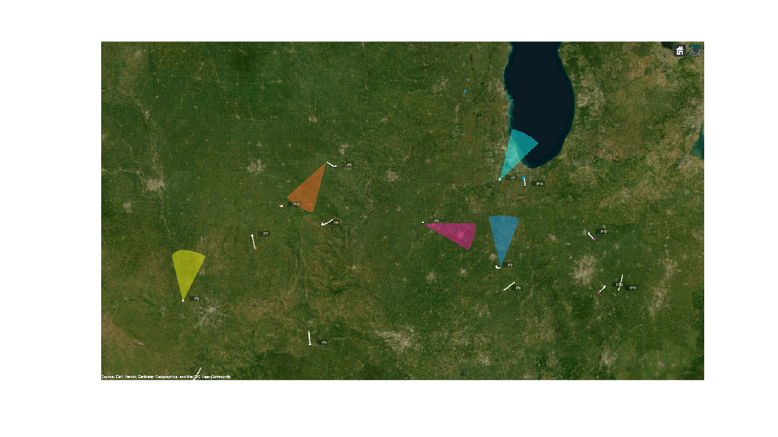
You visualize the recorded sensor data, truth data, and the tracker's estimates on a globe using the trackingGlobeViewer. The viewer is created using a supporting function defined at the bottom of this example. The image below shows the ground truth and spatial location of each sensor along with a conical coverage defining its field of view. Note that the range of the coverage is truncated for improved visibility of truth and detection data.
% Create globe viewer
viewer = createDisplay(sensorSpecs, sensorDataLog, truthDataLog);
f = figure('Units','normalized','Position',[0.1 0.1 0.8 0.8]);
img = snapshot(viewer);
ax = axes(f);
imshow(img,'Parent',ax);
You also quantitatively assess the performance of the tracking algorithm using the Optimal Sub Pattern Assignment (OSPA) metric using the trackOSPAMetric class.
% Quantitative metrics using OSPA
ospaMetric = trackOSPAMetric('Metric','OSPA',...
    'Distance','posnees');
ospa = zeros(numel(sensorDataLog), 1);
Now, you loop through the sensor data and iteratively update the tracker to obtain estimated tracks. You compute the OSPA metric by comparing the track data with truth data, and you update the display with new information.
for i = 1:numel(sensorDataLog)
    % Sensor data in current time interval
    sensorData = sensorDataLog{i};

    % Truth data in current time interval
    truthData = truthDataLog{i};

    % Update tracker with data in the current time interval
    tracks = tracker(sensorData{:});

    % Compute OSPA metric with trackable truths
    ospa(i) = ospaMetric(tracks, truthData(4:end));

    % Display
    updateDisplay(viewer, sensorSpecs, sensorData, tracks, truthData);
end
Results
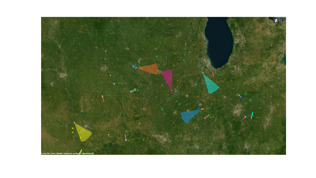
In the visualization used, the truth data is plotted in white, the detections of each sensor is plotted in the same color as their coverage cones, and the estimated tracks are plotted with a green line. The image below shows all the data captured from the radars during the scenario. Notice that the sensors reported several false alarms in addition to target measurements during the scenario.
figure('Units','normalized','Position',[0.1 0.1 0.8 0.8]);
snapshot(viewer);
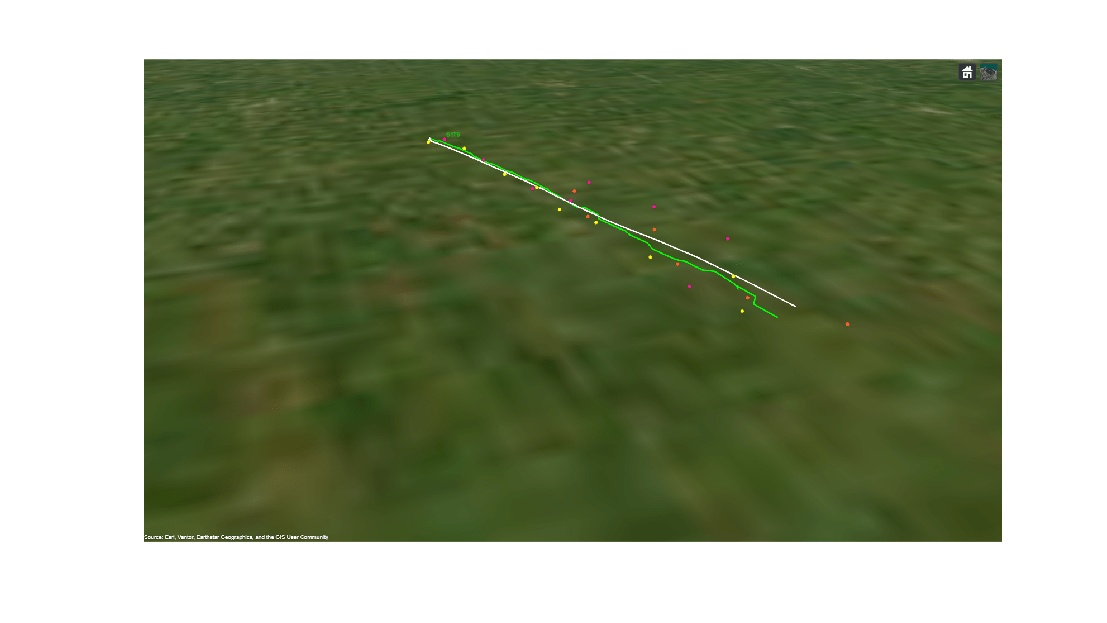
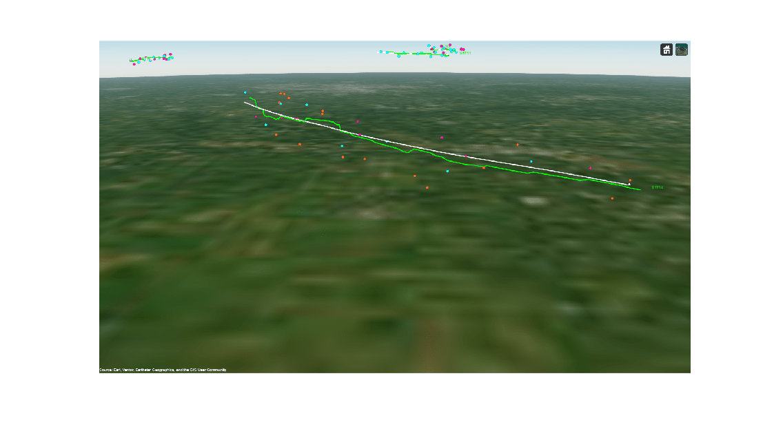
The image below shows the detections, true trajectories, and estimated trajectories of a few targets in a close-up view. Notice that the tracker is able to consistently maintain an estimate close to the actual trajectory of the object. Also note that the target was observed by different sensors in the scenario; this demonstrates that the tracker is able to handle the necessary coordinate transforms involved to fuse information from spatially distributed sensors in a geo-referenced environment.
campos(viewer, [40.100,-93.7413,2e4]);
camorient(viewer,[20.794 -27.13 0]);
f = figure('Units','normalized','Position',[0.1 0.1 0.8 0.8]);
img = snapshot(viewer);
ax = axes(f);
imshow(img,'Parent',ax);
campos(viewer, [39.573,-88.16,13737]);
camorient(viewer,[87.36 -18.49 0.085]);
f = figure('Units','normalized','Position',[0.1 0.1 0.8 0.8]);
img = snapshot(viewer);
ax = axes(f);
imshow(img,'Parent',ax);
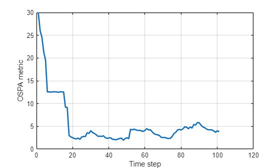
You also quantitatively assess the performance of the tracker by plotting the OSPA metric captured during tracking. The OSPA metric is a cost metric defined for a tracker and a lower value represents better tracking performance. Note that the OSPA metric remained low after the tracker established a track on each of the targets. This represents that the tracker was able to maintain an accurate track on each target without confirming false tracks.
figure();
plot(ospa,'LineWidth',2);
grid('on');
xlabel('Time step');
ylabel('OSPA metric');
Summary
In this example, you learned how to use the task-oriented approach to define and configure a JIPDA tracker for wide area surveillance applications that require tracking using geo-reference data. You fused recorded data from ground based and airborne radars for situational awareness in a large geographic scenario. You also learned how the target and sensor specifications alleviate the need for manual coordinate conversions between multiple frames involved in the tracking algorithm.
Supporting Functions
function viewer = createDisplay(sensorSpecs, sensorDataLog, truthDataLog)
% Create globe viewer
fig = uifigure('Units','normalized','Position',[0.1 0.1 0.8 0.8]);
viewer = trackingGlobeViewer(fig,'NumCovarianceSigma',0);

% Position the camera
campos(viewer,[40.9254,-90.2835,1e6]);

% Plot truth log to visualize entire trajectories beforehand
for i = 1:numel(truthDataLog)
    plotPlatform(viewer, truthDataLog{i}, 'ECEF', 'Color',[1 1 1],'LineWidth',2, 'TrajectoryMode','History');
end

% Create sensor data plotter to remove persistent detections
clear('helperPlotSensorData');

helperPlotSensorData(viewer, sensorSpecs, sensorDataLog{1},...
    PersistentDetections=true,...
    PlotCoverage=true,...
    DetectionHistoryTime=inf);

pause(2);
end

function updateDisplay(viewer, sensorSpecs, sensorData, tracks, truthData)
% Plot track data
plotTrack(viewer, tracks, 'ECEF','Color',[0 1 0],'LineWidth',2, 'MarkerSize',2);

% Plot truth data
plotPlatform(viewer, truthData, 'ECEF', 'Color',[1 1 1],'LineWidth',2,'TrajectoryMode','None', 'LabelStyle','None');

% Plot sensor measurements and coverage
helperPlotSensorData(viewer, sensorSpecs, sensorData,...
    PersistentDetections=true,...
    PlotCoverage=true,...
    DetectionHistoryTime=inf);
end