Implement Fuzzy Gain-Scheduled PID Controllers
This example shows how to implement fuzzy gain-scheduled control in a Simulink® model with a PID controller. This example tunes a fuzzy PID gain scheduler using genetic algorithm and pattern search algorithms, which require Global Optimization Toolbox software.
This example builds on the work done in Implement Gain-Scheduled PID Controllers (Simulink Control Design). In that example, the continuous stirred-tank reactor (CSTR) plant model is controlled with a gain-scheduled configuration, where the model uses multiple steady-state operating points for different output concentrations C = 2, 3, ..., 8, 9. The example uses the pidtune function to generate separate sets of PID coefficient (gain) values for each linearized model at different steady-state operating points and uses multiple 1-D Lookup Table blocks, as shown below, to implement gain-scheduled PID controllers.
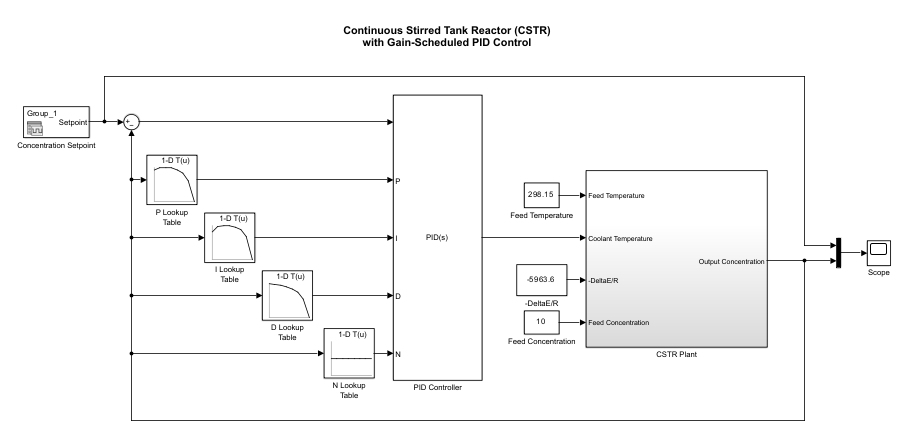
In this case, the lookup tables use the output concentration value as an input and generate PID coefficient values, which are connected to a PID Controller block. In the gain-scheduled configuration, the PID gains change as the output concentration changes, which ensures good PID control at any output concentration within the operating range of the control system.
This example tunes a fuzzy gain scheduler and compares its performance with the with the lookup table-based gain scheduler. The performance is compared using the integral of absolute error (IAE).
Load the example data.
data = load("FPIDGainSchedExample.mat");This model uses two gain-scheduling methods, which you can select by setting the schedulerType workspace variable to one of these values:
gainLookupTable— Select the lookup table-based gain scheduler.fuzzyGain— Select the fuzzy gain scheduler.
gainLookupTable = 1;
fuzzyGain = 2;
This example simulates gain schedulers using two reference setpoint trajectories. To select a trajectory for simulation, set the setpointPattern workspace variable to one of these values:
trainingSetpoints— This reference trajectory steps through a sequence of setpoints across the operating range of the system. These setpoints correspond to the operating points used for linearizing the plant model in the original example. In this example, you use this reference trajectory for tuning the rules and parameters of the fuzzy gain scheduler.testSetpoints— To validate controller performance against the nonlinear plant, this reference trajectory applies a series of steps of different sizes and directions across the operating range. In this example, you use this reference trajectory to test the robustness of the tuned fuzzy gain scheduler.
trainingSetpoints = 1;
testSetpoints = 2;
Open the model.
model = "FuzzyPIDGainSchedCSTRExampleModel";
open_system(model)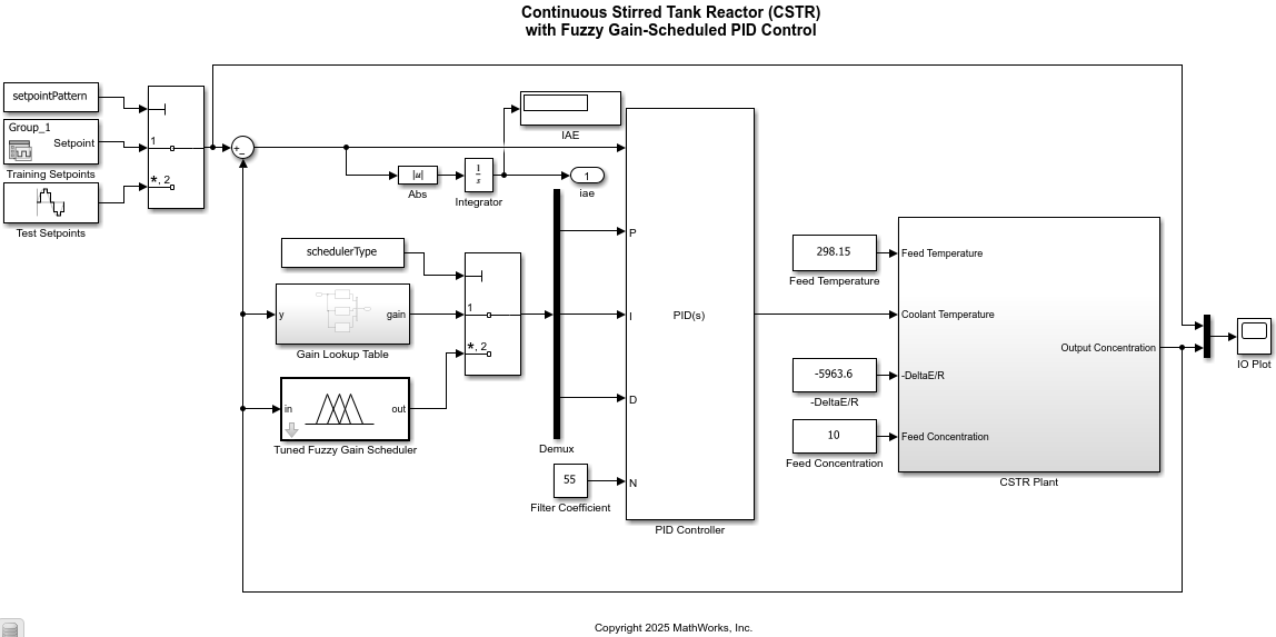
Gain Lookup Table
The Gain Lookup Table subsystem uses the same lookup tables as shown in the first figure for the PID gain values. In this case, the filter coefficient (N) lookup table is replaced with a constant block with a value of 55, which is similar to the filter coefficient of the original example. Simulate the model with the lookup table method using the training reference trajectory. To simulate the model, use the simWith helper function included at the end of this example. This function configures the scheduler and reference trajectory before simulating the model.
simOut = simWith(model,trainingSetpoints,gainLookupTable);
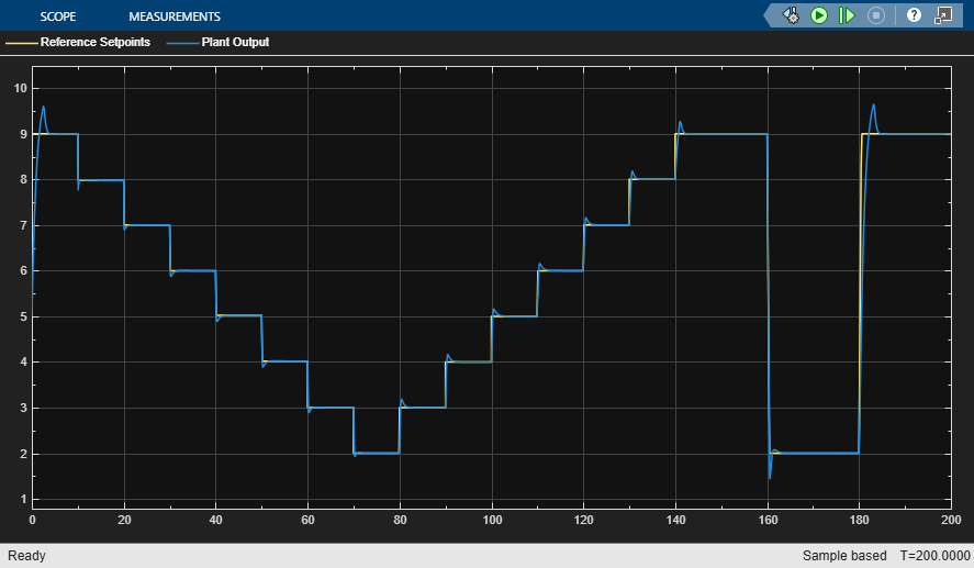
For this setpoint pattern, the performance metric value is:
IAE = simOut.yout(end)
IAE =
10.6765
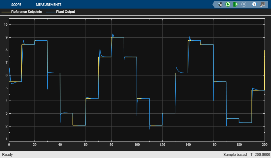
To check robustness of the method, simulate the model using the testing reference trajectory, which was not used during model linearization.
simOut = simWith(model,testSetpoints,gainLookupTable);
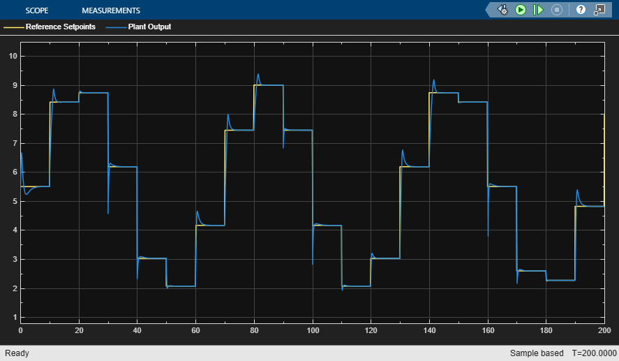
In this case, the overall error is higher compared to the training trajectory since the testing trajectory uses setpoints that were no originally used for model linearization.
IAE = simOut.yout(end)
IAE =
13.3043
Tuned Fuzzy Gain Scheduler
This approach uses available lookup table data from the original example to create an initial FIS for PID gain scheduling. The FIS parameters are then optimized using simulations to improve its IAE performance.
Construct an initial FIS using the controller data and setpoints. For FIS construction details, see the createInitialFISForTuning helper function included at the end of this example.
initialFIS = createInitialFISForTuning(data);
You can also load a presaved FIS.
initialFIS = readfis("InitialGainScheduler.fis");
The following figure shows the initial FIS construction.
figure
plotfis(initialFIS)
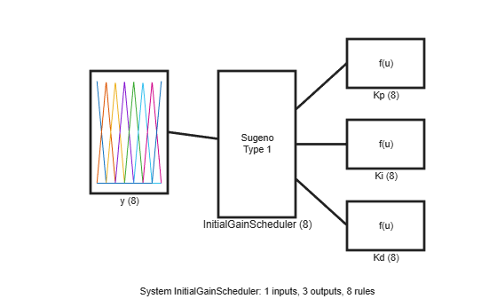
The FIS generates PID gain values for different output concentrations similar to the lookup table approach. The input range and membership function (MF) parameters are set based on the output concentration values.
figure
plotmf(initialFIS,"input",1)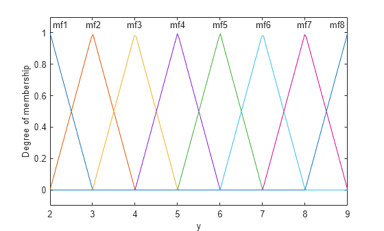
Input triangular MFs use peak values that match the lookup table output concentrations. For each FIS output, the singleton (constant) MFs are defined based on the corresponding lookup table data.
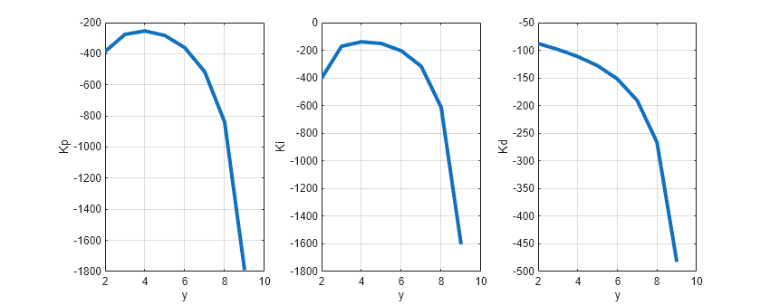
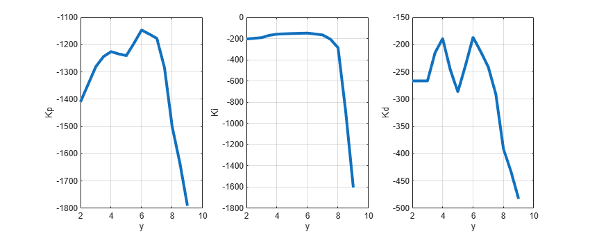
The rule base of the initial FIS defines the following input-output relations, which are similar to the lookup table representations shown in the first figure. To plot these figures, use the plotControlSurface helper function included at the end of this example.
plotControlSurface(initialFIS)
For faster simulation, this block uses a lookup table representation of the FIS with 80 input breakpoints. To use this configuration, set the following parameter values for the Tuned Fuzzy Gain Scheduler block:
Select the Implement FIS as lookup table parameter.
Set the Number of input breakpoints parameter to
80.
Simulate the model with this initial fuzzy gain scheduler using the training setpoint pattern.
gainScheduler = initialFIS;
simOut = simWith(model,trainingSetpoints,fuzzyGain);

In this case, the performance metric value is similar to the lookup table approach.
IAE = simOut.yout(end)
IAE =
10.6780
Next, to check the robustness of the fuzzy gain scheduler, simulate the model using the testing setpoint trajectory.
simOut = simWith(model,testSetpoints,fuzzyGain);

As with to the lookup table approach, the performance metric value deteriorates for the test pattern.
IAE = simOut.yout(end)
IAE =
13.2949
Tune Rule Parameters
Since the lookup table approach uses linearized models for PID gain coefficient calculation for different output concentrations, the performance can potentially be improved by optimizing the FIS parameters.
Tune the rule parameters to optimize the input-output relations of initialFIS. Optimize only the rule consequents since the rule antecedents use standard input MF combinations. Create a tunable settings object and set the rule antecedents as nontunable parameters.
[~,~,rules] = getTunableSettings(initialFIS);
for id = 1:numel(rules)
    rules(id).Antecedent.Free = false;
end
Create a tuning option set for genetic algorithm-based optimization. Set population size to 25, maximum generations to 100, and maximum stall generation to 10.
options = tunefisOptions(Method="ga");
options.MethodOptions.PopulationSize = 25;
options.MethodOptions.MaxGenerations = 100;
options.MethodOptions.MaxStallGenerations = 10;
Use a cost function to minimize the IAE performance metric. This cost function:
Simulates the nonlinear Simulink model using a candidate FIS object.
Uses the linearization setpoint pattern for its simulation.
function cost = fuzzyPIDGainSchedulingCostFcn(fis)
...
fisName = "gainScheduler";
model = "FuzzyPIDGainSchedCSTRExampleModel";
...
assignin("base",fisName,fis)
assignin("base","setpointPattern",1)
assignin("base","schedulerType",2)
out = sim(model);
iae = out.yout(end);
cost = iae;
...
end
Tune the FIS rules using the tunefis function. To load a pretuned FIS, set runtunefis to false.
runtunefis = false;
For tuning, initialize random number generator to the default algorithm and seed.
if runtunefis
    rng("default")
    ruleTunedFIS = tunefis(initialFIS,rules,@fuzzyPIDGainSchedulingCostFcn,options);
    ruleTunedFIS.Name = "GainSchedulerRuleTuned";
else
    ruleTunedFIS = readfis("GainSchedulerRuleTuned.fis");
end
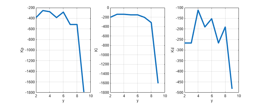
The tuned rule base generates the following input-output plots.
plotControlSurface(ruleTunedFIS)
Simulate the model with the tuned fuzzy gain scheduler. Use the training setpoint pattern for simulation.
gainScheduler = ruleTunedFIS;
simOut = simWith(model,trainingSetpoints,fuzzyGain);

In this case, the performance of ruleTunedFIS improves compared to initialFIS.
IAE = simOut.yout(end)
IAE =
9.6983
Next, simulate the model with the test setpoint pattern.
simOut = simWith(model,testSetpoints,fuzzyGain);
The performance using the test setpoint pattern also improves relative to initialFIS.
IAE = simOut.yout(end)
IAE =
12.4673
Tune Membership Function Parameters
Tune the input-output MF parameter values of the fuzzy system. To avoid overtuning the parameter values, use a local optimization method with a reduced maximum number of iterations. For this example use the pattern search method.
options.Method = "patternsearch";
options.MethodOptions.MaxIterations = 25;
Tune the MF parameter values.
if runtunefis
    rng("default")
    [ins,outs] = getTunableSettings(ruleTunedFIS);
    mfTunedFIS = tunefis(ruleTunedFIS,[ins;outs],@fuzzyPIDGainSchedulingCostFcn,options);
    mfTunedFIS.Name = "GainSchedulerMFTuned";
else
    mfTunedFIS = readfis("GainSchedulerMFTuned.fis");
end
The tuned MF parameters produce the following input-output plots.
plotControlSurface(mfTunedFIS)
Simulate the model with the tuned MF parameters using the training setpoint pattern.
gainScheduler = mfTunedFIS;
simOut = simWith(model,trainingSetpoints,fuzzyGain);
In this case, the performance of mfTunedFIS further improves compared to ruleTunedFIS.
IAE = simOut.yout(end)
IAE =
9.1895
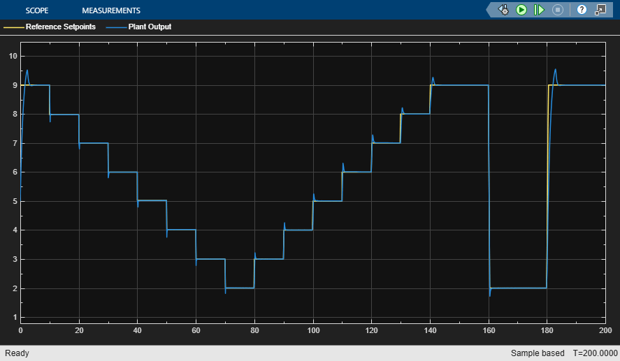
Next, validate the performance of mfTunedFIS using the test setpoint pattern.
simOut = simWith(model,testSetpoints,fuzzyGain);

In this case, the IAE performance of mfTunedFIS also improves compared to the ruleTunedFIS performance.
IAE = simOut.yout(end)
IAE =
12.1371
The plant output, however, includes higher peak values at the step changes, which indicates that the performance metric requires additional constraints to optimize the fuzzy system for a desired plant output.
Next Steps
To improve performance, you can consider the following next steps.
Use a Mamdani FIS with nonlinear MFs, such as Gaussian MFs, for smoother input-output mappings.
Use type-2 MFs to improve robustness for varying setpoints.
Use different setpoint patterns to improve the robustness of a tuned gain scheduler.
Investigate other optimization methods, such as particle swarm optimization, and random number generator seeds for performance variation.
Add additional costs to the performance metric to optimize additional signal attributes, such as overshoot or rise time.
Add additional inputs to the fuzzy system, such as error and change in error values, to produce robust controller gains for different setpoint patterns.
Local Functions
function simOut = simWith(model,setpointPattern,schedulerType)
% Simulates model with the specified scheduler type.

assignin("base","setpointPattern",setpointPattern)
assignin("base","schedulerType",schedulerType)
scope = model + "/IO Plot";
set_param(scope,"Visible","on")
simOut = sim(model);
end
function plotControlSurface(fis)
% Plot control surface for each output.
h = figure;
h.Position(3) = 850;
subplot(1,3,1)
gensurf(fis,gensurfOptions(OutputIndex=1))
subplot(1,3,2)
gensurf(fis,gensurfOptions(OutputIndex=2))
subplot(1,3,3)
gensurf(fis,gensurfOptions(OutputIndex=3))
end
function fis = createInitialFISForTuning(data)
% Creates an initial FIS for tuning.

controller = data.controllers;
setpoints = data.setpoints;

% Construct FIS
fis = sugfis(Name="InitialGainScheduler", ...
    AndMethod="min", ...
    OrMethod="max");

% Input 1
range = [min(setpoints) max(setpoints)];
fis = addInput(fis,range,Name="y");
fis = addMF(fis,"y","linzmf",[0 1]+range(1), ...
    Name="mf1",VariableType="input");
fis = addMF(fis,"y","trimf",[0 1 2]+range(1), ...
    Name="mf2",VariableType="input");
fis = addMF(fis,"y","trimf",[1 2 3]+range(1), ...
    Name="mf3",VariableType="input");
fis = addMF(fis,"y","trimf",[2 3 4]+range(1), ...
    Name="mf4",VariableType="input");
fis = addMF(fis,"y","trimf",[3 4 5]+range(1), ...
    Name="mf5",VariableType="input");
fis = addMF(fis,"y","trimf",[4 5 6]+range(1), ...
    Name="mf6",VariableType="input");
fis = addMF(fis,"y","trimf",[5 6 7]+range(1), ...
    Name="mf7",VariableType="input");
fis = addMF(fis,"y","linsmf",[6 7]+range(1), ...
    Name="mf8",VariableType="input");

% Output 1
Kp = sort(controller.Kp);
fis = addOutput(fis,[Kp(1) Kp(end)],Name="Kp");
fis = addMF(fis,"Kp","constant",Kp(1), ...
    Name="mf1",VariableType="output");
fis = addMF(fis,"Kp","constant",Kp(2), ...
    Name="mf2",VariableType="output");
fis = addMF(fis,"Kp","constant",Kp(3), ...
    Name="mf3",VariableType="output");
fis = addMF(fis,"Kp","constant",Kp(4), ...
    Name="mf4",VariableType="output");
fis = addMF(fis,"Kp","constant",Kp(5), ...
    Name="mf5",VariableType="output");
fis = addMF(fis,"Kp","constant",Kp(6), ...
    Name="mf6",VariableType="output");
fis = addMF(fis,"Kp","constant",Kp(7), ...
    Name="mf7",VariableType="output");
fis = addMF(fis,"Kp","constant",Kp(8), ...
    Name="mf8",VariableType="output");

% Output 2
Ki = sort(controller.Ki);
fis = addOutput(fis,[Ki(1) Ki(end)],Name="Ki");
fis = addMF(fis,"Ki","constant",Ki(1), ...
    Name="mf1",VariableType="output");
fis = addMF(fis,"Ki","constant",Ki(2), ...
    Name="mf2",VariableType="output");
fis = addMF(fis,"Ki","constant",Ki(3), ...
    Name="mf3",VariableType="output");
fis = addMF(fis,"Ki","constant",Ki(4), ...
    Name="mf4",VariableType="output");
fis = addMF(fis,"Ki","constant",Ki(5), ...
    Name="mf5",VariableType="output");
fis = addMF(fis,"Ki","constant",Ki(6), ...
    Name="mf6",VariableType="output");
fis = addMF(fis,"Ki","constant",Ki(7), ...
    Name="mf7",VariableType="output");
fis = addMF(fis,"Ki","constant",Ki(8), ...
    Name="mf8",VariableType="output");

% Output 3
Kd = sort(controller.Kd);
fis = addOutput(fis,[Kd(1) Kd(end)],Name="Kd");
fis = addMF(fis,"Kd","constant",Kd(1), ...
    Name="mf1",VariableType="output");
fis = addMF(fis,"Kd","constant",Kd(2), ...
    Name="mf2",VariableType="output");
fis = addMF(fis,"Kd","constant",Kd(3), ...
    Name="mf3",VariableType="output");
fis = addMF(fis,"Kd","constant",Kd(4), ...
    Name="mf4",VariableType="output");
fis = addMF(fis,"Kd","constant",Kd(5), ...
    Name="mf5",VariableType="output");
fis = addMF(fis,"Kd","constant",Kd(6), ...
    Name="mf6",VariableType="output");
fis = addMF(fis,"Kd","constant",Kd(7), ...
    Name="mf7",VariableType="output");
fis = addMF(fis,"Kd","constant",Kd(8), ...
    Name="mf8",VariableType="output");

% Rules
fis = addRule(fis,[ ...
    "y==mf1 => Kp=mf4, Ki=mf3, Kd=mf8 (1)" ...
    "y==mf2 => Kp=mf7, Ki=mf6, Kd=mf7 (1)" ...
    "y==mf3 => Kp=mf8, Ki=mf8, Kd=mf6 (1)" ...
    "y==mf4 => Kp=mf6, Ki=mf7, Kd=mf5 (1)" ...
    "y==mf5 => Kp=mf5, Ki=mf5, Kd=mf4 (1)" ...
    "y==mf6 => Kp=mf3, Ki=mf4, Kd=mf3 (1)" ...
    "y==mf7 => Kp=mf2, Ki=mf2, Kd=mf2 (1)" ...
    "y==mf8 => Kp=mf1, Ki=mf1, Kd=mf1 (1)"] ...
    );

end
See Also
Topics
- Tuning Fuzzy Inference Systems
- Implement Gain-Scheduled PID Controllers (Simulink Control Design)