Performing a Multiobjective Optimization Using the Genetic Algorithm

R2026b

This example shows how to perform a multiobjective optimization using multiobjective genetic algorithm function gamultiobj in Global Optimization Toolbox.

Simple Multiobjective Optimization Problem

gamultiobj can be used to solve multiobjective optimization problem in several variables. Here we want to minimize two objectives, each having one decision variable.

$$\underset{x}{\min }F(x)=[objective1(x);objective2(x)]$$

where

$$\begin{array}{l}objective1(x)=(x+2{)}^2-10\\ objective2(x)=(x-2{)}^2-20.\end{array}$$

Plot the two objective functions.

x = -10:0.5:10;
f1 = (x+2).^2 - 10;
f2 = (x-2).^2 + 20;
plot(x,f1);
hold on;
plot(x,f2,"r");
grid on;
title("Plot of objectives (x+2)^2 - 10 and (x-2)^2 + 20");

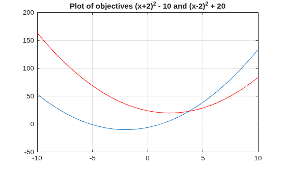
The two objectives have their minima at $$x=-2$$ and $$x=+2$$ respectively. However, in a multiobjective problem, $$x=-2$$, $$x=2$$, and any solution in the range $$-2<=x<=2$$ is equally optimal. There is no single solution to this multiobjective problem. The goal of the multiobjective genetic algorithm is to find a set of solutions in that range (ideally with a good spread). The set of solutions is also known as a Pareto front. All solutions on the Pareto front are optimal.

Coding the Fitness Function

Create a MATLAB® file named simple_multiobjective.m:

function y = simple_multiobjective(x)
y(1) = (x+2)^2 - 10;
y(2) = (x-2)^2 + 20;
end

The Genetic Algorithm solver assumes the fitness function will take one input $$x$$, where $$x$$ is a row vector with as many elements as the number of variables in the problem. The fitness function computes the value of each objective function and returns these values in a single vector output $$y$$.

Minimizing Using gamultiobj

To use the gamultiobj function, we need to provide at least two input arguments, a fitness function, and the number of variables in the problem. The first two output arguments returned by gamultiobj are x, the points on Pareto front, and fval, the objective function values at the values x. A third output argument, exitflag, tells you the reason why gamultiobj stopped. A fourth argument, output, contains information about the performance of the solver. gamultiobj can also return a fifth argument, population, that contains the population when gamultiobj terminated and a sixth argument, score, that contains the function values of all objectives for population when gamultiobj terminated.

FitnessFunction = @simple_multiobjective;
numberOfVariables = 1;
[x,fval] = gamultiobj(FitnessFunction,numberOfVariables);

gamultiobj stopped because it exceeded options.MaxGenerations.

The x returned by the solver is a matrix in which each row is the point on the Pareto front for the objective functions. The fval is a matrix in which each row contains the value of the objective functions evaluated at the corresponding point in x.

size(x)

ans = 1×2

    18     1

size(fval)

ans = 1×2

    18     2

Constrained Multiobjective Optimization Problem

gamultiobj can handle optimization problems with linear inequality, equality, and simple bound constraints. Here we want to add bound constraints on simple multiobjective problem solved previously.

$$\underset{x}{\min }F(x)=[objective1(x);objective2(x)]$$

subject to $$-1.5\le x\le 0$$ (bound constraints)

where

$$\begin{array}{l}objective1(x)=(x+2{)}^2-10\\ objective2(x)=(x-2{)}^2-20.\end{array}$$

gamultiobj accepts linear inequality constraints in the form $$Ax\le b$$ and linear equality constraints in the form $$Aeqx=beq$$ and bound constraints in the form $$lb\le x\le ub$$. We pass $$A$$ and $$Aeq$$ as matrices and $$b$$, $$beq$$, $$lb$$, and $$ub$$ as vectors. Since we have no linear constraints in this example, we pass [] for those inputs.

A = []; b = [];
Aeq = []; beq = [];
lb = -1.5;
ub = 0;
x = gamultiobj(FitnessFunction,numberOfVariables,A,b,Aeq,beq,lb,ub);

gamultiobj stopped because it exceeded options.MaxGenerations.

All solutions in x (each row) will satisfy all linear and bound constraints within the tolerance specified in options.ConstraintTolerance. However, if you use your own crossover or mutation function, ensure that the new individuals are feasible with respect to linear and simple bound constraints.

Adding Visualization

gamultiobj can accept one or more plot functions through the options argument. This feature is useful for visualizing the performance of the solver at run time. Plot functions can be selected using optimoptions.

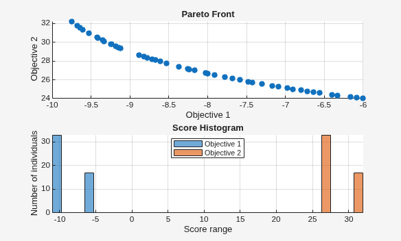
Here we use optimoptions to select two plot functions. The first plot function is gaplotpareto, which plots the Pareto front (limited to any three objectives) at every generation. The second plot function is gaplotscorediversity, which plots the score diversity for each objective. The options are passed as the last argument to the solver.

options = optimoptions(@gamultiobj,PlotFcn={@gaplotpareto,@gaplotscorediversity});
gamultiobj(FitnessFunction,numberOfVariables,[],[],[],[],lb,ub,options);

gamultiobj stopped because it exceeded options.MaxGenerations.

Vectorizing Your Fitness Function

Consider the previous fitness functions again:

$$\begin{array}{l}objective1(x)=(x+2{)}^2-10\\ objective2(x)=(x-2{)}^2-20.\end{array}$$

By default, the gamultiobj solver only passes in one point at a time to the fitness function. However, if the fitness function is vectorized to accept a set of points and returns a set of function values you can speed up your solution.

For example, if the solver needs to evaluate five points in one call to this fitness function, then it will call the function with a matrix of size 5-by-1, i.e., 5 rows and 1 column (recall that 1 is the number of variables).

Create a MATLAB file called vectorized_multiobjective.m:

function scores = vectorized_multiobjective(pop)
popSize = size(pop,1); % Population size 
numObj = 2;  % Number of objectives
% initialize scores
scores = zeros(popSize, numObj);
% Compute first objective
scores(:,1) = (pop + 2).^2 - 10;
% Compute second objective
scores(:,2) = (pop - 2).^2 + 20;
end

This vectorized version of the fitness function takes a matrix |pop| with an arbitrary number of points, the rows of pop, and returns a matrix of size populationSize-by- numberOfObjectives.

We need to specify that the fitness function is vectorized using the options created using optimoptions. The options are passed in as the ninth argument.

FitnessFunction = @(x)vectorized_multiobjective(x);
options = optimoptions(@gamultiobj,UseVectorized=true);
gamultiobj(FitnessFunction,numberOfVariables,[],[],[],[],lb,ub,options);

gamultiobj stopped because the average change in the spread of Pareto solutions is less than options.FunctionTolerance.