Isolated Global Minimum
Difficult-To-Locate Global Minimum
Finding a start point in the basin of attraction of the global minimum can be difficult when the basin is small or when you are unsure of the location of the minimum. To solve this type of problem you can:
Add sensible bounds
Take a huge number of random start points
Make a methodical grid of start points
For an unconstrained problem, take widely dispersed random start points
This example shows these methods and some variants.
The function is nearly zero for all , and .The example is a two-dimensional version of the sech function, with one minimum at [1,1], the other at [1e5,-1e5]:
has a global minimum of –21 at (1e5,–1e5), and a local minimum of –11 at (1,1).
x1 = [1,1]; x2 = [1e5,-1e5];
% f is a vectorized version of the objective function
% Each row of an input matrix x is one point to evaluate
f = @(x,y)-10*sech(sqrt((x-x1(1)).^2+(y-x1(2)).^2)) ...
    -20*sech(3e-4*sqrt((x-x2(1)).^2+(y-x2(2)).^2))-1;
hndl = fsurf(@(x,y)f(x,y),[-1e6 1e6]);
zlim([-20,0])
set(hndl,LineStyle="none")
view(-45,10)
hold on
annotation("textarrow",...
    [0.71 0.56],[0.48 0.21],TextEdgeColor="none",...
    String="Global Minimum");
annotation("textarrow",...
    [.4,.52],[.6,.6],TextEdgeColor="none",...
    String="Local Minimum");
hold off
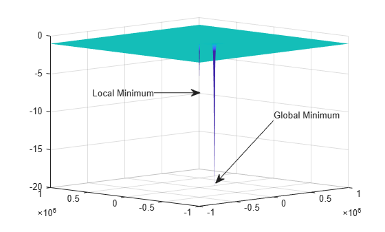
The minimum at (1e5,–1e5) shows as a narrow spike. The minimum at (1,1) does not show completely because it is too narrow.
The following sections show various methods of searching for the global minimum. Some of the methods are not successful on this problem. Nevertheless, you might find each method useful for different problems.
Default Settings Cannot Find the Global Minimum — Add Bounds
GlobalSearch and MultiStart cannot find the global minimum using default global options, since the default start point components are in the range (–9999,10001) for GlobalSearch and (–1000,1000) for MultiStart.
With additional bounds of –1e6 and 1e6 in problem, GlobalSearch usually does not find the global minimum:
x1 = [1;1];x2 = [1e5;-1e5];
f = @(x)-10*sech(norm(x(:)-x1)) -20*sech((norm(x(:)-x2))*3e-4) -1;
opts = optimoptions(@fmincon,Algorithm="active-set");
problem = createOptimProblem("fmincon",x0=[0,0],objective=f,...
    lb=[-1e6;-1e6],ub=[1e6;1e6],options=opts);
gs = GlobalSearch;
rng(14,"twister") % For reproducibility
[xfinal,fval] = run(gs,problem)
GlobalSearch stopped because it analyzed all the trial points.

All 32 local solver runs converged with a positive local solver exit flag.
xfinal = 1×2

    1.0000    1.0000
fval =
-11.0000
GlobalSearch with Bounds and More Start Points
To find the global minimum, you can search more points. This example uses 1e5 start points, and a MaxTime of 300 s:
gs.NumTrialPoints = 1e5;
gs.MaxTime = 300;
[xg,fvalg] = run(gs,problem)
GlobalSearch stopped because it analyzed all the trial points.

4389 out of 4941 local solver runs converged with a positive local solver exit flag.
xg = 1×2
104 ×

   10.0000  -10.0000
fvalg =
-21.0000
In this case, GlobalSearch finds the global minimum.
MultiStart with Bounds and Many Start Points
Alternatively, you can search using MultiStart with many start points. This example uses 1e5 start points, and a MaxTime of 300 s:
ms = MultiStart(gs);
[xm,fvalm] = run(ms,problem,1e5)
MultiStart completed some of the runs from the start points.

99996 out of 100000 local solver runs converged with a positive local solver exitflag.
xm = 1×2

    1.0000    1.0000
fvalm =
-11.0000
In this case, MultiStart fails to find the global minimum.
MultiStart Without Bounds, Widely Dispersed Start Points
You can also use MultiStart to search an unbounded region to find the global minimum. Again, you need many start points to have a good chance of finding the global minimum.
The first five lines of code generate 10,000 widely dispersed random start points using the method described in . newprob is a problem structure using the fminunc local solver and no bounds:
rng(0,"twister") % for reproducibility
u = rand(1e4,1);
u = 1./u;
u = exp(u) - exp(1);
s = rand(1e4,1)*2*pi;
stpts = [u.*cos(s),u.*sin(s)];
startpts = CustomStartPointSet(stpts);

opts = optimoptions(@fminunc,Algorithm="quasi-newton");
newprob = createOptimProblem("fminunc",x0=[0;0],objective=f,...
    options=opts);
[xcust,fcust] = run(ms,newprob,startpts)
MultiStart completed the runs from all start points.

All 10000 local solver runs converged with a positive local solver exitflag.
xcust = 2×1
105 ×

    1.0000
   -1.0000
fcust =
-21.0000
In this case, MultiStart finds the global minimum.
MultiStart with a Regular Grid of Start Points
You can also use a grid of start points instead of random start points. To learn how to construct a regular grid for more dimensions, or one that has small perturbations, see Uniform Grid or Perturbed Grid.
xx = -1e6:1e4:1e6;
[xxx,yyy] = meshgrid(xx,xx);
z = [xxx(:),yyy(:)];
bigstart = CustomStartPointSet(z);
[xgrid,fgrid] = run(ms,newprob,bigstart)
MultiStart completed the runs from all start points.

All 40401 local solver runs converged with a positive local solver exitflag.
xgrid = 2×1

      100000
     -100000
fgrid =
-21
In this case, MultiStart finds the global minimum.
MultiStart with Regular Grid and Promising Start Points
Making a regular grid of start points, especially in high dimensions, can use an inordinate amount of memory or time. You can filter the start points to run only those with small objective function value.
To perform this filtering most efficiently, write your objective function in a vectorized fashion. For information, see Write a Vectorized Function or Vectorize the Objective and Constraint Functions. The following function handle computes a vector of objectives based on an input matrix whose rows represent start points:
x1 = [1;1];x2 = [1e5;-1e5];
g = @(x) -10*sech(sqrt((x(:,1)-x1(1)).^2 + (x(:,2)-x1(2)).^2)) ...
    -20*sech(sqrt((x(:,1)-x2(1)).^2 + (x(:,2)-x2(2)).^2))-1;
Suppose you want to run the local solver only for points where the value is less than –2. Start with a denser grid than in internal link, then filter out all the points with high function value:
xx = -1e6:1e3:1e6;
[xxx,yyy] = meshgrid(xx,xx);
z = [xxx(:),yyy(:)];
idx = g(z) < -2; % index of promising start points
zz = z(idx,:);
smallstartset = CustomStartPointSet(zz);
opts = optimoptions(@fminunc,Algorithm="quasi-newton",Display="off");
newprobg = createOptimProblem("fminunc",x0=[0,0],...
    objective=g,options=opts);
% row vector x0 since g expects rows
[xfew,ffew] = run(ms,newprobg,smallstartset)
MultiStart completed the runs from all start points.

All 2 local solver runs converged with a positive local solver exitflag.
xfew = 1×2

      100000     -100000
ffew =
-21
In this case, MultiStart finds the global minimum. There are only two start points in smallstartset, one of which is the global minimum.