Estimate SISO State-Space Model Using AAA Algorithm
This example demonstrates how to identify a state-space model to fit the frequency response of a building vibration using the Adaptive Antoulas-Anderson (AAA) algorithm within the ssest function. It estimates the model from a single-input single-output (SISO) frequency-domain data set. The example also estimates state-space models using the least-squares rational function (LSRF) and subspace state-space (N4SID) estimation algorithms and then compares all the estimated models.
Data Preparation
To generate the frequency-domain data set, first load a state-space model with one input, one output, and 48 hidden states.
load build.mat G
To reproduce results of this example, use a random number seed.
rng("default")Now, generate the training and validation data sets. To generate each data set:
frequency_train = logspace(0,3,2000);
response_train = freqresp(G,frequency_train);
data_train = idfrd(response_train,frequency_train,0);

frequency_val = logspace(0,2.5,1000);
response_val = freqresp(G,frequency_val);
data_val = idfrd(response_val,frequency_val,0);
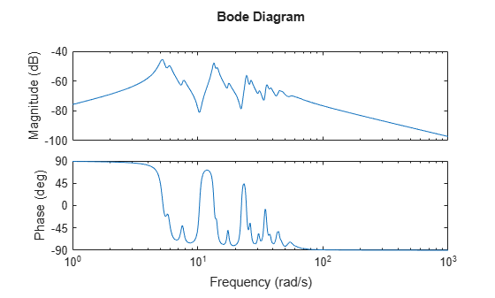
You can visualize the training data set using the bode command.
bode(data_train)
Model Estimation Using AAA Algorithm
To initialize the state-space parameters using the AAA algorithm, specify the InitializeMethod property of the ssestOptions option set as 'AAA'. To disable the nonlinear optimization that occurs after the AAA algorithm stops and to display the results obtained only from the AAA algorithm, set the MaxIterations property to be 0. Optionally, you can enable further fine-tuning of the results by setting the MaxIterations property to a positive integer.
opt_aaa = ssestOptions;
opt_aaa.InitializeMethod = 'AAA';
opt_aaa.SearchOptions.MaxIterations = 0;
Specify the limit on the number of poles in the model, nx. In each iteration, the AAA algorithm adds a real pole or a pair of complex-conjugate poles to the identified model until this limit is reached or until the fitting error is below AAATolerance. So, for a SISO system, the order of the estimated model will be less than or equal to (nx+1). For more information on the AAA algorithm and the error tolerance, see the InitializeMethod property and the AAATolerance option under the Advanced property of the ssestOptions object.
nx = 8;
Estimate a continuous-time state-space model using the training data set and the specified options.
sys_aaa = ssest(data_train,nx,'Ts',data_train.Ts,opt_aaa)sys_aaa =
Continuous-time identified state-space model:
dx/dt = A x(t) + B u(t) + K e(t)
y(t) = C x(t) + D u(t) + e(t)
A =
x1 x2 x3 x4 x5 x6 x7 x8
x1 -0.9774 24.5 0 0 0 0 0 0
x2 -24.5 -0.9774 0 0 0 0 0 0
x3 0 0 -0.4461 13.48 0 0 0 0
x4 0 0 -13.48 -0.4461 0 0 0 0
x5 0 0 0 0 -0.2647 5.239 0 0
x6 0 0 0 0 -5.239 -0.2647 0 0
x7 0 0 0 0 0 0 -0.29 5.87
x8 0 0 0 0 0 0 -5.87 -0.29
B =
u1
x1 0.2781
x2 0.2005
x3 -0.1914
x4 0.2632
x5 -0.2443
x6 0.04306
x7 0.1576
x8 0.2064
C =
x1 x2 x3 x4 x5 x6 x7 x8
y1 0.005825 0.006675 -0.008291 0.007803 -0.01059 0.001935 0.002182 0.00471
D =
u1
y1 0
K =
y1
x1 0
x2 0
x3 0
x4 0
x5 0
x6 0
x7 0
x8 0
Parameterization:
STRUCTURED form (some fixed coefficients in A, B, C).
Feedthrough: none
Disturbance component: none
Number of free coefficients: 32
Use "idssdata", "getpvec", "getcov" for parameters and their uncertainties.
Status:
Estimated using SSEST on frequency response data "data_train".
Fit to estimation data: 83.55%
FPE: 2.694e-08, MSE: 2.651e-08
Model Properties
Model Estimation Using LSRF Algorithm
To initialize the state-space parameters using the LSRF algorithm, specify the InitializeMethod property of the ssestOptions option set as 'lsrf' and the MaxIterations property as false.
opt_lsrf = ssestOptions;
opt_lsrf.InitializeMethod = 'lsrf';
opt_lsrf.SearchOptions.MaxIterations = 0;
Specify the order of the estimated model, nx_lsrf.
nx_lsrf = 8;
Estimate a continuous-time state-space model using the training data set and the specified options.
sys_lsrf = ssest(data_train,nx_lsrf,'Ts',data_train.Ts,opt_lsrf)sys_lsrf =
Continuous-time identified state-space model:
dx/dt = A x(t) + B u(t) + K e(t)
y(t) = C x(t) + D u(t) + e(t)
A =
x1 x2 x3 x4 x5 x6 x7 x8
x1 -0.2629 5.256 0 0 0 0 0 0
x2 -5.256 -0.2629 -1.162 -0.9799 -9.762 -1.429 -8.224 -1.888
x3 0 0 -0.2989 11.63 0 0 0 0
x4 0 0 -2.908 -0.2989 -1.528 -0.2236 -1.287 -0.2954
x5 0 0 0 0 -0.5502 13.55 0 0
x6 0 0 0 0 -13.55 -0.5502 -5.034 -1.155
x7 0 0 0 0 0 0 -0.8854 24.46
x8 0 0 0 0 0 0 -24.46 -0.8854
B =
u1
x1 0
x2 0.06273
x3 0
x4 0.009816
x5 0
x6 0.0384
x7 0
x8 0.03284
C =
x1 x2 x3 x4 x5 x6 x7 x8
y1 -0.02011 0.1649 0 0 0 0 0 0
D =
u1
y1 0
K =
y1
x1 0
x2 0
x3 0
x4 0
x5 0
x6 0
x7 0
x8 0
Parameterization:
FREE form (all coefficients in A, B, C free).
Feedthrough: none
Disturbance component: none
Number of free coefficients: 80
Use "idssdata", "getpvec", "getcov" for parameters and their uncertainties.
Status:
Estimated using SSEST on frequency response data "data_train".
Fit to estimation data: 85.27%
FPE: 2.159e-08, MSE: 2.124e-08
Model Properties
Model Estimation Using N4SID Algorithm
To initialize the state-space parameters using the N4SID algorithm, specify the InitializeMethod property of the ssestOptions option set as 'n4sid' and the MaxIterations property as false.
opt_n4sid = ssestOptions;
opt_n4sid.InitializeMethod = 'n4sid';
opt_n4sid.SearchOptions.MaxIterations = 0;
Specify the order of the estimated model, nx_n4sid.
nx_n4sid = 8;
Estimate a continuous-time state-space model using the training data set and the specified options.
sys_n4sid = ssest(data_train,nx_n4sid,'Ts',data_train.Ts,opt_n4sid)sys_n4sid =
Continuous-time identified state-space model:
dx/dt = A x(t) + B u(t) + K e(t)
y(t) = C x(t) + D u(t) + e(t)
A =
x1 x2 x3 x4 x5 x6 x7 x8
x1 -0.5439 57.15 -1.229 -87.17 1.861 114.3 -2.177 -143.3
x2 -1.116 -5.387 127.9 14.8 -176.2 -13.94 223.7 15.92
x3 -0.008119 -1.552 -0.02194 -200.1 0.3715 257.9 -0.04697 -323.4
x4 0.01231 -0.2186 3.545 -9.645 276.6 17.37 -348.1 -19.18
x5 -0.0002754 0.00532 -0.004463 -2.51 -0.4691 -362.6 0.6085 451
x6 8.293e-05 -0.001518 0.001311 -0.1379 3.015 -6.01 459 11.94
x7 -4.659e-07 7.753e-06 -3.044e-06 0.000926 -0.0014 -2.31 -0.01438 -574.7
x8 3.333e-07 -6.127e-06 6.881e-06 -0.0005476 0.001151 -0.04849 2.024 -5.458
B =
u1
x1 -0.001724
x2 0.0001102
x3 0.0005422
x4 7.998e-05
x5 1.888e-05
x6 2.004e-06
x7 1.169e-07
x8 7.727e-09
C =
x1 x2 x3 x4 x5 x6 x7 x8
y1 -4.072 7.376 -9.037 -11.32 12.62 14.48 -16 -18.05
D =
u1
y1 0
K =
y1
x1 0
x2 0
x3 0
x4 0
x5 0
x6 0
x7 0
x8 0
Parameterization:
FREE form (all coefficients in A, B, C free).
Feedthrough: none
Disturbance component: none
Number of free coefficients: 80
Use "idssdata", "getpvec", "getcov" for parameters and their uncertainties.
Status:
Estimated using SSEST on frequency response data "data_train".
Fit to estimation data: 6.499%
FPE: 8.702e-07, MSE: 8.564e-07
Model Properties
Model Refinement Using Numerical Search
You can improve the estimated models by using numerical search algorithms.
In this example, fine-tune the model sys_aaa using the Levenberg–Marquardt least squares search approach. For more information, see the SearchMethod property of ssestOptions.
opt_aaa.SearchMethod = "lm";
opt_aaa.SearchOptions.MaxIterations = 100;
sys_aaa_improved = ssest(data_train,sys_aaa,opt_aaa)
sys_aaa_improved =
Continuous-time identified state-space model:
dx/dt = A x(t) + B u(t) + K e(t)
y(t) = C x(t) + D u(t) + e(t)
A =
x1 x2 x3 x4 x5 x6 x7 x8
x1 -0.8853 24.46 0 0 0 0 0 0
x2 -24.46 -0.8853 0 0 0 0 0 0
x3 0 0 -0.5504 13.55 0 0 0 0
x4 0 0 -13.55 -0.5504 0 0 0 0
x5 0 0 0 0 -0.2628 5.256 0 0
x6 0 0 0 0 -5.256 -0.2628 0 0
x7 0 0 0 0 0 0 -0.299 5.816
x8 0 0 0 0 0 0 -5.816 -0.299
B =
u1
x1 0.278
x2 0.2005
x3 -0.1914
x4 0.2632
x5 -0.2443
x6 0.04302
x7 0.1577
x8 0.2064
C =
x1 x2 x3 x4 x5 x6 x7 x8
y1 0.004312 0.005349 -0.008794 0.009069 -0.01046 0.002867 0.001447 0.005327
D =
u1
y1 0
K =
y1
x1 0
x2 0
x3 0
x4 0
x5 0
x6 0
x7 0
x8 0
Parameterization:
STRUCTURED form (some fixed coefficients in A, B, C).
Feedthrough: none
Disturbance component: none
Number of free coefficients: 32
Use "idssdata", "getpvec", "getcov" for parameters and their uncertainties.
Status:
Estimated using SSEST on frequency response data "data_train".
Fit to estimation data: 85.27%
FPE: 2.159e-08, MSE: 2.124e-08
Model Properties
Comparison of Results
Calculate the fit percentages of all the estimated models.
fit_aaa = sys_aaa.Report.Fit.FitPercent
fit_aaa =
83.5484
fit_lsrf = sys_lsrf.Report.Fit.FitPercent
fit_lsrf =
85.2737
fit_n4sid = sys_n4sid.Report.Fit.FitPercent
fit_n4sid =
6.4995
fit_aaa_improved = sys_aaa_improved.Report.Fit.FitPercent
fit_aaa_improved =
85.2737
For the data used in this example, the AAA and LSRF algorithms return similar results which are better when compared to the N4SID algorithm.
Plot the responses of the state-space models estimated using the AAA, LSRF, and N4SID algorithms over the validation data set. Also plot the response of the improved model.
compare(data_val,sys_aaa,sys_lsrf,sys_n4sid,sys_aaa_improved)
legend("show",Interpreter="none")
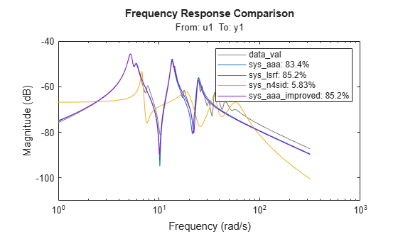
You can verify that the models estimated using the AAA and LSRF algorithms have similar responses and both these models outperform the model estimated using the N4SID algorithm. The improved model performs better than the initial model estimated using AAA algorithm.
See Also
ssestOptions | ssest | bode | compare