Spectrum Analyzer Plot
This example shows how to use the Quick Control Spectrum Analyzer to acquire power spectrum data from a Keysight® Technologies N9040B spectrum analyzer.
Introduction
This example uses a spectrum analyzer to acquire power spectrum data within the Bluetooth® band of 2.402 GHz to 2.48 GHz.
Requirements
To run this example, you need:
Keysight Technologies N9040B spectrum analyzer
IVI-C driver for Keysight Technologies N9040B spectrum analyzer (AgXSAn)
NI™ VISA or Keysight VISA
NI IVI® compliance package version 16.0.1.2 or higher
Create an RF Spectrum Analyzer Object
Create the Quick Control object and search for available resources and drivers.
rfsa = rfspecan;
resources(rfsa)
ans =
    ' TCPIP0::K-N9040B-91124.dhcp.mathworks.com::inst0::INSTR
     '
drivers(rfsa)
ans =
    'Driver: AgXSAn
     Supported Models:
        M8920A, M90XA, M9290A, M9410A, M9411A, M9415A, M9420A
        M9421A, N8973B, N8974B, N8975B, N8976B, N9000A, N9000B
        N9010A, N9010B, N9020A, N9020B, N9021B, N9030A, N9030B
        N9032B, N9038A, N9038B, N9040B, N9041B, N9042B, N9048B

     Driver: rsspecan
     Supported Models:
     ESW, FPH, FPS, FSV, FSVA, FSVR, FSW, FSWP, FSWT

     '
Connect to the Selected Resource and Driver
Select an available resource and driver.
rfsa.Resource = "TCPIP0::K-N9040B-91124.dhcp.mathworks.com::inst0::INSTR";
rfsa.Driver = "AgXSAn";
connect(rfsa)
disp(rfsa)
  RFSpecAn with properties:

                Resource: "TCPIP0::K-N9040B-91124.dhcp.mathworks.com::inst0::INSTR"
                  Driver: "AgXSAn"
                  Vendor: "Keysight Technologies"
                   Model: "N9040B"
          StartFrequency: 10000000
           StopFrequency: 2.6500e+10
         CenterFrequency: 1.3255e+10
                    Span: 2.6490e+10
               SweepTime: 0.0665
     ResolutionBandwidth: 3000000
          VideoBandwidth: 3000000
           VerticalScale: Logarithmic
          AmplitudeUnits: dBm
          ReferenceLevel: 0
    ReferenceLevelOffset: 0

  Show all properties, functions
Configure the Start and Stop Frequencies
Set the start frequency to just below the start of the Bluetooth band of 2.402 GHz. Set the stop frequency to just above the end of the Bluetooth band of 2.48 GHz.
rfsa.StartFrequency = 2.4e9;
rfsa.StopFrequency = 2.5e9
  RFSpecAn with properties:

                Resource: "TCPIP0::K-N9040B-91124.dhcp.mathworks.com::inst0::INSTR"
                  Driver: "AgXSAn"
                  Vendor: "Keysight Technologies"
                   Model: "N9040B"
          StartFrequency: 2.4000e+09
           StopFrequency: 2.5000e+09
         CenterFrequency: 2.4500e+09
                    Span: 100000000
               SweepTime: 1.0000e-03
     ResolutionBandwidth: 910000
          VideoBandwidth: 910000
           VerticalScale: Logarithmic
          AmplitudeUnits: dBm
          ReferenceLevel: 0
    ReferenceLevelOffset: 0

  Show all properties, functions
Acquire Power Spectrum Amplitude Data
Acquire 100 real-valued power spectra. Each spectrum has a number of points equal to the TraceSize, which is a fixed value for the N9040B.
n = 100;
data = nan(rfsa.TraceSize, n);
for i = 1:n
    data(:, i) = readPowerSpectrum(rfsa);
end
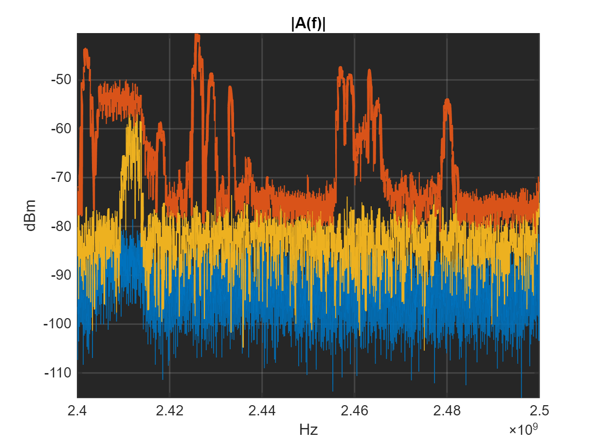
Plot the Average and the Envelope of the Acquired Data
This is effectively the same as acquiring using "Minimum Hold" and "Maximum Hold" trace types.
Amin = min(data, [], 2);
Amax = max(data, [], 2);
Amean = mean(data, 2);

f = linspace(rfsa.StartFrequency, rfsa.StopFrequency, rfsa.TraceSize);

figure;
hold on

plot(f, Amin, LineWidth=2);
plot(f, Amax, LineWidth=2);
plot(f, Amean, LineWidth=2);

title("|A(f)|")
% Label using the current units of amplitude, which are set to "dBm" by
% default.
ylabel(string(rfsa.AmplitudeUnits));
xlabel("Hz")

setAxesSpectrumAnalyzer(gca);

Live Plot the Current Data and Trace the Maximum and Minimum Hold
Display the data as observed on a front-panel display using three traces (sample, minimum, and maximum).
figure;

Amin = data(:, 1);
Amax = data(:, 1);
Anext = data(:, 1);

p = plot(f, Amin, f, Anext, f, Amax, LineWidth=2);
ax = gca;
setAxesSpectrumAnalyzer(ax)
colors = colororder;
order = [1 3 2];
ax.ColorOrder = colors(order, :);

title("|A(f)|")
ylabel(string(rfsa.AmplitudeUnits));
xlabel("Hz")

axis tight

p(1).YDataSource =  'Amin';
p(2).YDataSource =  'Anext';
p(3).YDataSource =  'Amax';

for i = 2:n
    Anext = data(:, i);
    Amin = min(Amin, Anext);
    Amax = max(Amax, Anext);

    axis tight
    refreshdata
    drawnow limitrate nocallbacks
    pause(0.100);
end
Front-Panel Display
function setAxesSpectrumAnalyzer(haxes)
% Configure the plot to look like a front-panel display
% of a stand-alone instrument.

set(haxes, 'Color', [0.150 0.150 0.150], ...
           'GridColor', [1 1 1], ...
           'GridLineWidth', 1, ...
           'XGrid','on', ...
           'YGrid','on');
end