Build Watts-Strogatz Small World Graph Model

R2026b

This example shows how to construct and analyze a Watts-Strogatz small-world graph. The Watts-Strogatz model is a random graph that has small-world network properties, such as clustering and short average path length.

Algorithm Description

Creating a Watts-Strogatz graph has two basic steps:

Create a ring lattice with $N$ nodes of mean degree $2 K$ . Each node is connect to its $K$ nearest neighbors on either side.
For each edge in the graph, rewire the target node with probability $β$ . The rewired edge cannot be a duplicate or self-loop.

After the first step the graph is a perfect ring lattice. So when $β = 0$ , no edges are rewired and the model returns a ring lattice. In contrast, when $β = 1$ , all of the edges are rewired and the ring lattice is transformed into a random graph.

The file WattsStrogatz.m implements this graph algorithm for undirected graphs. The input parameters are N, K, and beta according to the algorithm description above.

View the file WattsStrogatz.m.

% Copyright 2015 The MathWorks, Inc.

function h = WattsStrogatz(N,K,beta)
% H = WattsStrogatz(N,K,beta) returns a Watts-Strogatz model graph with N
% nodes, N*K edges, mean node degree 2*K, and rewiring probability beta.
%
% beta = 0 is a ring lattice, and beta = 1 is a random graph.

% Connect each node to its K next and previous neighbors. This constructs
% indices for a ring lattice.
s = repelem((1:N)',1,K);
t = s + repmat(1:K,N,1);
t = mod(t-1,N)+1;

% Rewire the target node of each edge with probability beta
for source=1:N    
    switchEdge = rand(K, 1) < beta;

    newTargets = rand(N, 1);
    newTargets(source) = 0;
    newTargets(s(t==source)) = 0;
    newTargets(t(source, ~switchEdge)) = 0;

    [~, ind] = sort(newTargets, 'descend');
    t(source, switchEdge) = ind(1:nnz(switchEdge));
end

h = graph(s,t);
end
a=1;

Ring Lattice

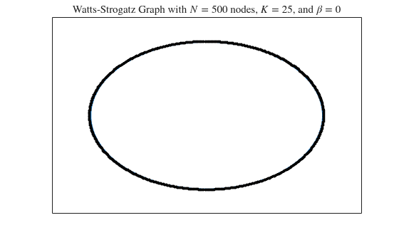
Construct a ring lattice with 500 nodes using the WattsStrogatz function. When beta is 0, the function returns a ring lattice whose nodes all have degree 2K.

h = WattsStrogatz(500,25,0);
plot(h,'NodeColor','k','Layout','circle');
title('Watts-Strogatz Graph with $N = 500$ nodes, $K = 25$, and $\beta = 0$', ...
    'Interpreter','latex')

Figure contains an axes object. The axes object with title Watts - Strogatz Graph with N equals 5 0 0 nodes, K equals 2 5 , and beta equals 0 contains an object of type graphplot.

Some Random Edges

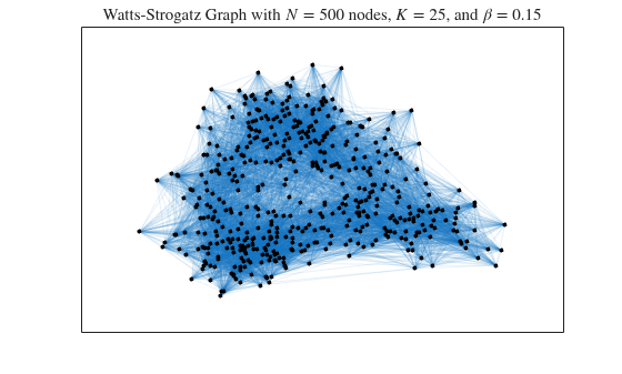
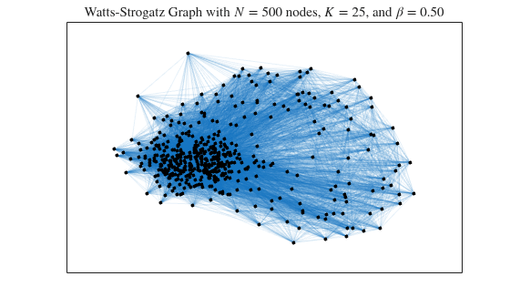
Increase the amount of randomness in the graph by raising beta to 0.15 and 0.50.

h2 = WattsStrogatz(500,25,0.15);
plot(h2,'NodeColor','k','EdgeAlpha',0.1);
title('Watts-Strogatz Graph with $N = 500$ nodes, $K = 25$, and $\beta = 0.15$', ...
    'Interpreter','latex')

Figure contains an axes object. The axes object with title Watts - Strogatz Graph with N equals 5 0 0 nodes, K equals 2 5 , and beta equals 0 point 1 5 contains an object of type graphplot.

h3 = WattsStrogatz(500,25,0.50);
plot(h3,'NodeColor','k','EdgeAlpha',0.1);
title('Watts-Strogatz Graph with $N = 500$ nodes, $K = 25$, and $\beta = 0.50$', ...
    'Interpreter','latex')

Figure contains an axes object. The axes object with title Watts - Strogatz Graph with N equals 5 0 0 nodes, K equals 2 5 , and beta equals 0 point 5 0 contains an object of type graphplot.

Random Graph

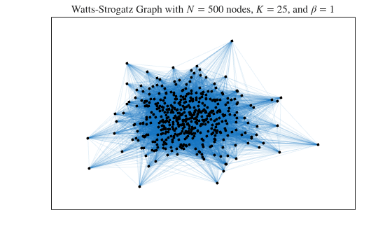
Generate a completely random graph by increasing beta to its maximum value of 1.0. This rewires all of the edges.

h4 = WattsStrogatz(500,25,1);
plot(h4,'NodeColor','k','EdgeAlpha',0.1);
title('Watts-Strogatz Graph with $N = 500$ nodes, $K = 25$, and $\beta = 1$', ...
    'Interpreter','latex')

Figure contains an axes object. The axes object with title Watts - Strogatz Graph with N equals 5 0 0 nodes, K equals 2 5 , and beta equals 1 contains an object of type graphplot.

Degree Distribution

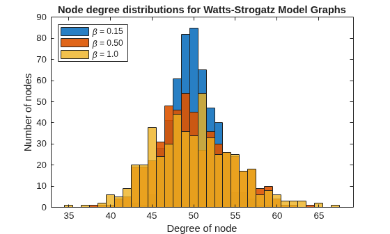
The degree distribution of the nodes in the different Watts-Strogatz graph varies. When beta is 0, the nodes all have the same degree, 2K, so the degree distribution is just a Dirac-delta function centered on 2K, $δ (x - 2 K)$ , However, as beta increases, the degree distribution changes.

This plot shows the degree distributions for the nonzero values of beta.

histogram(degree(h2),'BinMethod','integers','FaceAlpha',0.9);
hold on
histogram(degree(h3),'BinMethod','integers','FaceAlpha',0.9);
histogram(degree(h4),'BinMethod','integers','FaceAlpha',0.8);
hold off
title('Node degree distributions for Watts-Strogatz Model Graphs')
xlabel('Degree of node')
ylabel('Number of nodes')
legend('\beta = 0.15','\beta = 0.50','\beta = 1.0','Location','NorthWest')

$Figure contains an axes object. The axes object with title Node degree distributions for Watts-Strogatz Model Graphs, xlabel Degree of node, ylabel Number of nodes contains 3 objects of type histogram. These objects represent \beta = 0.15, \beta = 0.50, \beta = 1.0.$

Hub Formation

The Watts-Strogatz graph has a high clustering coefficient, so the nodes tend to form cliques, or small groups of closely interconnected nodes. As beta increases towards its maximum value of 1.0, you see an increasingly large number of hub nodes, or nodes of high relative degree. The hubs are a common connection between other nodes and between cliques in the graph. The existence of hubs is what permits the formation of cliques while preserving a short average path length.

Calculate the average path length and number of hub nodes for each value of beta. For the purposes of this example, the hub nodes are nodes with degree greater than or equal to 55. These are all of the nodes whose degree increased 10% or more compared to the original ring lattice.

n = 55;
d = [mean(mean(distances(h))), nnz(degree(h)>=n); ...
    mean(mean(distances(h2))), nnz(degree(h2)>=n); ...
    mean(mean(distances(h3))), nnz(degree(h3)>=n);
    mean(mean(distances(h4))), nnz(degree(h4)>=n)];
T = table([0 0.15 0.50 1]', d(:,1), d(:,2),...
    'VariableNames',{'Beta','AvgPathLength','NumberOfHubs'})

T = 4×3 table
    Beta    AvgPathLength    NumberOfHubs
    ____    _____________    ____________

       0         5.48              0     
    0.15       2.0715             20     
     0.5       1.9101             85     
       1       1.9008             92

As beta increase, the average path length in the graph quickly falls to its limiting value. This is due to the formation of the highly connected hub nodes, which become more numerous as beta increases.

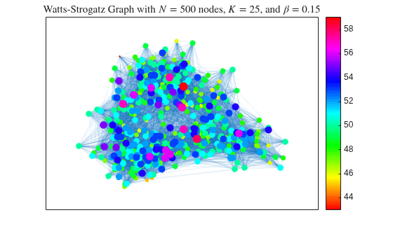
Plot the $β = 0.15$ Watts-Strogatz model graph, making the size and color of each node proportional to its degree. This is an effective way to visualize the formation of hubs.

deg = degree(h2);
nSizes = 2*sqrt(deg-min(deg)+0.2);
nColors = deg;
plot(h2,'MarkerSize',nSizes,'NodeCData',nColors,'EdgeAlpha',0.1)
title('Watts-Strogatz Graph with $N = 500$ nodes, $K = 25$, and $\beta = 0.15$', ...
    'Interpreter','latex')
colorbar
colormap hsv