Solve BVP Using Continuation
This example shows how to solve a numerically difficult boundary value problem using continuation, which effectively breaks the problem up into a sequence of simpler problems.
For , consider the differential equation
.
The problem is posed on the interval and is subject to the boundary conditions
,
.
When , the solution to the equation undergoes a rapid transition near , so it is difficult to solve numerically. Instead, this example uses continuation to iterate through several values of until . The intermediate solutions are each used as the initial guess for the next problem.
To solve this system of equations in MATLAB®, you need to code the equations, boundary conditions, and initial guess before calling the boundary value problem solver bvp4c. You either can include the required functions as local functions at the end of a file (as done here), or you can save them as separate, named files in a directory on the MATLAB path.
Code Equation
Using the substitutions and , you can rewrite the equation as the system of first-order equations
,
.
Write a function to code the equations with the signature dydx = shockode(x,y), where:
xis the independent variable.yis the dependent variable.dydx(1)gives the equation for , anddydx(2)gives the equation for .
Make the function vectorized, so that shockode([x1 x2 ...],[y1 y2 ...]) returns [shockode(x1,y1) shockode(x2,y2) ...]. This approach improves solver performance.
The corresponding function is
function dydx = shockode(x,y)
pix = pi*x;
dydx = [y(2,:)
       -x/e.*y(2,:) - pi^2*cos(pix) - pix/e.*sin(pix)];
end
Note: All functions are included as local functions at the end of the example.
Code Boundary Conditions
The BVP solver requires the boundary conditions to be in the form . In this form the boundary conditions are:
,
.
Write a function to code the boundary conditions with the signature res = shockbc(ya,yb), where:
yais the value of the boundary condition at the beginning of the interval .ybis the value of the boundary condition at the end of the interval .
The corresponding function is
function res = shockbc(ya,yb) % boundary conditions
res = [ya(1)+2
       yb(1)];
end
Code Jacobians
The analytical Jacobians for the ODE function and boundary conditions can be calculated easily in this problem. Providing the Jacobians makes the solver more efficient, since the solver no longer needs to approximate them with finite differences.
For the ODE function, the Jacobian matrix is
.
The corresponding function is
function jac = shockjac(x,y,e)
jac = [0   1
       0  -x/e];
end
Similarly, for the boundary conditions, the Jacobian matrices are
, .
The corresponding function is
function [dBCdya,dBCdyb] = shockbcjac(ya,yb)
dBCdya = [1 0; 0 0];
dBCdyb = [0 0; 1 0];
end
Form Initial Guess
Use a constant guess for the solution on a mesh of five points in .
sol = bvpinit([-1 -0.5 0 0.5 1],[1 0]);
Solve Equation
If you try to solve the equation directly using , then the solver is not able to overcome the poor conditioning of the problem near the transition point. Instead, to obtain the solution for , this example uses continuation by solving a sequence of problems for , , and . The output from the solver in each iteration acts as the guess for the solution in the next iteration (this is why the variable for the initial guess from bvpinit is sol, and the output from the solver is also named sol).
Since the value of the Jacobian depends on the value of , set the options in the loop specifying the shockjac and shockbcjac functions for the Jacobians. Also, turn vectorization on since shockode is coded to handle vectors of values.
e = 0.1;
for i = 2:4
   e = e/10;
   options = bvpset('FJacobian',@(x,y) shockjac(x,y,e),...
                    'BCJacobian',@shockbcjac,...
                    'Vectorized','on');
   sol = bvp4c(@(x,y) shockode(x,y,e),@shockbc, sol, options);
end
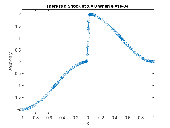
Plot Solution
Plot the results from bvp4c for the mesh and solution . With continuation, the solver is able to handle the discontinuity at .
plot(sol.x,sol.y(1,:),'-o');
axis([-1 1 -2.2 2.2]);
title(['There Is a Shock at x = 0 When e =' sprintf('%.e',e) '.']);
xlabel('x');
ylabel('solution y');
Local Functions
Listed here are the local functions that the BVP solver bvp4c calls to calculate the solution. Alternatively, you can save these functions as their own files in a directory on the MATLAB path.
function dydx = shockode(x,y,e) % equation to solve
pix = pi*x;
dydx = [y(2,:)
       -x/e.*y(2,:) - pi^2*cos(pix) - pix/e.*sin(pix)];
end
%-------------------------------------------
function res = shockbc(ya,yb) % boundary conditions
res = [ya(1)+2
       yb(1)];
end
%-------------------------------------------
function jac = shockjac(x,y,e) % jacobian of shockode
jac = [0   1
       0  -x/e];
end
%-------------------------------------------
function [dBCdya,dBCdyb] = shockbcjac(ya,yb) % jacobian of shockbc
dBCdya = [1 0; 0 0];
dBCdyb = [0 0; 1 0];
end
%-------------------------------------------