Solve BVP with Multiple Boundary Conditions
This example shows how to solve a multipoint boundary value problem, where the solution of interest satisfies conditions inside the interval of integration.
For in , consider the equations
,
.
The known parameters of the problem are , , , and .
The term in the equation for is not smooth at , so the problem cannot be solved directly. Instead, you can break the problem into two: one set in the interval , and the other set in the interval . The connection between the two regions is that the solutions must be continuous at . The solution must also satisfy the boundary conditions
,
.
The equations for each region are
Region 1:
,
.
Region 2:
,
.
The interface point is included in both regions. At this point, the solver produces both left and right solutions, which must be equal to ensure continuity of the solution.
To solve this system of equations in MATLAB®, you need to code the equations, boundary conditions, and initial guess before calling the boundary value problem solver bvp5c. You either can include the required functions as local functions at the end of a file (as done here), or save them as separate, named files in a directory on the MATLAB path.
Code Equations
The equations for and depend on the region being solved. For multipoint boundary value problems the derivative function must accept a third input argument region, which is used to identify the region where the derivative is being evaluated. The solver numbers the regions from left to right, starting with 1.
Create a function to code the equations with the signature dydx = f(x,y,region,p), where:
xis the independent variable.yis the dependent variable.dydx(1)gives the equation for , anddydx(2)the equation for .regionis the number of the region where the derivative is being computed (in this two-region problem,regionis1or2).pis a vector containing the values of the constant parameters .
Use a switch statement to return different equations depending on the region being solved. The function is
function dydx = f(x,y,region,p) % equations being solved
n = p(1);
eta = p(4);

dydx = zeros(2,1);
dydx(1) = (y(2) - 1)/n;

switch region
    case 1    % x in [0 1]
        dydx(2) = (y(1)*y(2) - x)/eta;
    case 2    % x in [1 lambda]
        dydx(2) = (y(1)*y(2) - 1)/eta;
end
end
Note: All functions are included as local functions at the end of the example.
Code Boundary Conditions
Solving two first-order differential equations in two regions requires four boundary conditions. Two of these conditions come from the original problem:
,
.
The other two conditions enforce the continuity of the left and right solutions at the interface point :
,
.
For multipoint BVPs, the arguments of the boundary conditions function YL and YR become matrices. In particular, the kth column YL(:,k) is the solution at the left boundary of the kth region. Similarly, YR(:,k) is the solution at the right boundary of the kth region.
In this problem, is approximated by YL(:,1), while is approximated by YR(:,end). Continuity of the solution at requires that YR(:,1) = YL(:,2).
The function that encodes the residual value of the four boundary conditions is
function res = bc(YL,YR)
res = [YL(1,1)               % v(0) = 0
       YR(1,1) - YL(1,2)     % Continuity of v(x) at x=1
       YR(2,1) - YL(2,2)     % Continuity of C(x) at x=1
       YR(2,end) - 1];       % C(lambda) = 1
end
Form Initial Guess
For multipoint BVPs, the boundary conditions are automatically applied at the beginning and end of the interval of integration. However, you must specify double entries in xmesh for the other interface points. A simple guess that satisfies the boundary conditions is the constant guess y = [1; 1].
xc = 1;
xmesh = [0 0.25 0.5 0.75 xc xc 1.25 1.5 1.75 2];
yinit = [1; 1];
sol = bvpinit(xmesh,yinit);
Solve Equation
Define the values of the constant parameters and put them in the vector p. Provide the function to bvp5c with the syntax @(x,y,r) f(x,y,r,p) to provide the vector of parameters.
Calculate the solution for several values of , using each solution as the initial guess for the next. For each value of , calculate the value of the osmolarity . For each iteration of the loop, compare the computed value with the approximate analytical solution.
lambda = 2;
n = 5e-2;
for kappa = 2:5
   eta = lambda^2/(n*kappa^2);
   p = [n kappa lambda eta];
   sol = bvp5c(@(x,y,r) f(x,y,r,p), @bc, sol);
   K2 = lambda*sinh(kappa/lambda)/(kappa*cosh(kappa));
   approx = 1/(1 - K2);
   computed = 1/sol.y(1,end);
   fprintf('  %2i    %10.3f     %10.3f \n',kappa,computed,approx);
end
   2         1.462          1.454
   3         1.172          1.164
   4         1.078          1.071
   5         1.039          1.034
Plot Solution
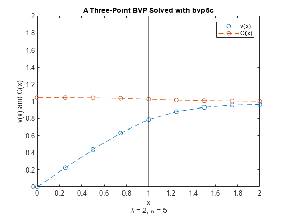
Plot the solution components for and and a vertical line at the interface point . The displayed solution for results from the final iteration of the loop.
plot(sol.x,sol.y(1,:),'--o',sol.x,sol.y(2,:),'--o')
line([1 1], [0 2], 'Color', 'k')
legend('v(x)','C(x)')
title('A Three-Point BVP Solved with bvp5c')
xlabel({'x', '\lambda = 2, \kappa = 5'})
ylabel('v(x) and C(x)')
Local Functions
Listed here are the local helper functions that the BVP solver bvp5c calls to calculate the solution. Alternatively, you can save these functions as their own files in a directory on the MATLAB path.
function dydx = f(x,y,region,p) % equations being solved
n = p(1);
eta = p(4);

dydx = zeros(2,1);
dydx(1) = (y(2) - 1)/n;

switch region
    case 1    % x in [0 1]
        dydx(2) = (y(1)*y(2) - x)/eta;
    case 2    % x in [1 lambda]
        dydx(2) = (y(1)*y(2) - 1)/eta;
end
end
%-------------------------------------------
function res = bc(YL,YR) % boundary conditions
res = [YL(1,1)               % v(0) = 0
       YR(1,1) - YL(1,2)     % Continuity of v(x) at x=1
       YR(2,1) - YL(2,2)     % Continuity of C(x) at x=1
       YR(2,end) - 1];       % C(lambda) = 1
end
%-------------------------------------------