Visualizing Volume Data
This example shows several methods for visualizing volume data in MATLAB®.
Display Isosurface
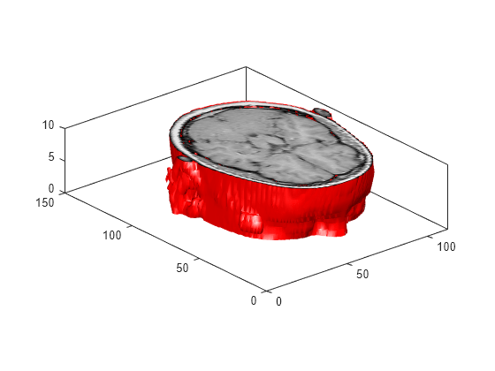
An isosurface is a surface where all the points within a volume of space have a constant value. Use the isosurface function to generate the faces and vertices for the outside of the surface and the isocaps function to generate the faces and vertices for the end caps of the volume. Use the patch command to draw the volume and its end caps.
load mri D
D = squeeze(D);
limits = [NaN NaN NaN NaN NaN 10]
limits = 1×6

   NaN   NaN   NaN   NaN   NaN    10
[x, y, z, D] = subvolume(D, limits);
[fo,vo] = isosurface(x,y,z,D,5);
[fe,ve,ce] = isocaps(x,y,z,D,5);
figure
p1 = patch('Faces', fo, 'Vertices', vo);
p1.FaceColor = 'red'
p1 =
  Patch with properties:

    FaceColor: [1 0 0]
    FaceAlpha: 1
    EdgeColor: [0.1294 0.1294 0.1294]
    LineStyle: '-'
        Faces: [23351×3 double]
     Vertices: [12406×3 double]

  Show all properties
p1.EdgeColor = 'none'p1 =
Patch with properties:
FaceColor: [1 0 0]
FaceAlpha: 1
EdgeColor: 'none'
LineStyle: '-'
Faces: [23351×3 double]
Vertices: [12406×3 double]
Show all properties
p2 = patch('Faces', fe, 'Vertices', ve, ...
   'FaceVertexCData', ce)
p2 =
  Patch with properties:

    FaceColor: [0.1294 0.1294 0.1294]
    FaceAlpha: 1
    EdgeColor: [0.1294 0.1294 0.1294]
    LineStyle: '-'
        Faces: [27265×3 double]
     Vertices: [14250×3 double]

  Show all properties
p2.FaceColor = 'interp';
p2.EdgeColor = 'none';

view(-40,24)
daspect([1 1 0.3])
colormap(gray(100))
box on

camlight(40,40)
camlight(-20,-10)
lighting gouraud

Create Cone Plot
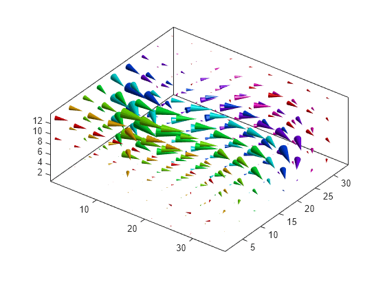
The coneplot command plots velocity vectors as cones at x, y, z points in a volume. The cones represent the magnitude and direction of the vector field at each point.
cla
load wind u v w x y z
[m,n,p] = size(u)
m =
35
n =
41
p =
15
[Cx, Cy, Cz] = meshgrid(1:4:m,1:4:n,1:4:p);
h = coneplot(u,v,w,Cx,Cy,Cz,y,4);
set(h,'EdgeColor', 'none')

axis tight equal
view(37,32)
box on
colormap(hsv)
light

Plot Streamlines
The streamline function plots streamlines for a velocity vector at x, y, z points in a volume to illustrate the flow of a 3-D vector field.
cla

[m,n,p] = size(u);
[Sx, Sy, Sz] = meshgrid(1,1:5:n,1:5:p);
streamline(u,v,w,Sx,Sy,Sz)

axis tight equal
view(37,32)
box on

Plot Streamtubes
The streamtube function plots streamtubes for a velocity vector at x, y, z points in a volume. The width of the tube is proportional to the normalized divergence of the vector field at each point.
cla

[~,n,p] = size(u);
[Sx, Sy, Sz] = meshgrid(1,1:5:n,1:5:p);
h = streamtube(u,v,w,Sx,Sy,Sz);
set(h, 'FaceColor', 'cyan')
set(h, 'EdgeColor', 'none')

axis tight equal
view(37,32)
box on
light

Combine Volume Visualizations
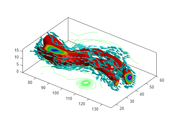
Combine volume visualization in a single plot to get a more comprehensive picture of a velocity field within a volume.
cla
spd = sqrt(u.*u + v.*v + w.*w);
[fo,vo] = isosurface(x,y,z,spd,40);
[fe,ve,ce] = isocaps(x,y,z,spd,40);
p1 = patch('Faces', fo, 'Vertices', vo);
p1.FaceColor = 'red'
p1 =
  Patch with properties:

    FaceColor: [1 0 0]
    FaceAlpha: 1
    EdgeColor: [0.1294 0.1294 0.1294]
    LineStyle: '-'
        Faces: [5340×3 double]
     Vertices: [2727×3 double]

  Show all properties
p1.EdgeColor = 'none'p1 =
Patch with properties:
FaceColor: [1 0 0]
FaceAlpha: 1
EdgeColor: 'none'
LineStyle: '-'
Faces: [5340×3 double]
Vertices: [2727×3 double]
Show all properties
p2 = patch('Faces', fe, 'Vertices', ve, ...
   'FaceVertexCData', ce)
p2 =
  Patch with properties:

    FaceColor: [0.1294 0.1294 0.1294]
    FaceAlpha: 1
    EdgeColor: [0.1294 0.1294 0.1294]
    LineStyle: '-'
        Faces: [464×3 double]
     Vertices: [301×3 double]

  Show all properties
p2.FaceColor = 'interp'p2 =
Patch with properties:
FaceColor: 'interp'
FaceAlpha: 1
EdgeColor: [0.1294 0.1294 0.1294]
LineStyle: '-'
Faces: [464×3 double]
Vertices: [301×3 double]
Show all properties
p2.EdgeColor = 'none' p2 =
Patch with properties:
FaceColor: 'interp'
FaceAlpha: 1
EdgeColor: 'none'
LineStyle: '-'
Faces: [464×3 double]
Vertices: [301×3 double]
Show all properties
[fc, vc] = isosurface(x, y, z, spd, 30);
[fc, vc] = reducepatch(fc, vc, 0.2);
h1 = coneplot(x,y,z,u,v,w,vc(:,1),vc(:,2),vc(:,3),3);
h1.FaceColor = 'cyan';
h1.EdgeColor = 'none';

[sx, sy, sz] = meshgrid(80, 20:10:50, 0:5:15);
h2 = streamline(x,y,z,u,v,w,sx,sy,sz);
set(h2, 'Color', [.4 1 .4])

axis tight equal
view(37,32)
box on
light
